|
|
Contents Introduction Overview of Deterministic algorithm Overview of Monte Carlo algorithm Scenes used for comparison Accuracy analysis Results obtained Conclusion Acknowledgments |
|
|
|
Contents Introduction Overview of Deterministic algorithm Overview of Monte Carlo algorithm Scenes used for comparison Accuracy analysis Results obtained Conclusion Acknowledgments |
|
The Monte Carlo global illumination algorithm used in TBT / SPECTER is an alternative to the deterministic algorithm described above. It provides results in the same form (i-maps described in sec. 2.3) as the Deterministic algorithm. A user can choose the method of global illumination analysis (it is also possible to run them both and then choose one of resultant i-maps for image generation).
The method is based on Forward Monte Carlo Ray Tracing. Forward means that we trace rays originated in light sources.
In few words, the method is the following. At first a light source is chosen randomly with probability proportional to its total luminous flux. In case of extended light sources a point on its surface is chosen randomly. Then a ray direction is chosen randomly in accordance with spatial distribution of light intensity of this source. (This spatial distribution is characterized in TBT by the so called goniometric diagram that determines luminous intensity of emitted light in each direction.)
The ray built is then traced until intersection with some scene element (or until it leaves the domain: enclosing box for the scene). When an intersection is found an event to be performed is selected, it may be specular / diffuse reflection / refraction, absorption, etc. A probability of each event is determined by appropriate reflectance / transmittance / absorption coefficients. If absorption is chosen we simply stop further tracing of this ray (the same for the rays leaving the scene). Otherwise a new ray direction is chosen deterministically (in case of specular event when next ray direction is unique) or stochastically (in case of diffuse scattering). In the last case probability distribution obeys the predefined characteristics of diffuse scattering of the surface met.
The characteristic feature of our algorithm is that we don't change the ray energy during its tracing. Each event that may change ray energy (a partial absorption in material or in surface) is treated in the probabilistic way, by the Russian Roulette Rule: either the ray survive with the unchanged energy or it completely disappears. By a proper choice of probabilities of these two events we can simulate any rate of light absorption. In this sense we follow the global idea of using a random choice everywhere without decrease of simulation accuracy. This idea was explicitly stated in [CPC84] (in application to Backward Monte Carlo ray tracing).
During Forward ray tracing ray-surface intersections are also processed from the viewpoint of i-maps calculation: if a ray hits a triangle that keeps i-maps then appropriate element(s) of the i-maps is modified to account for energy brought by the ray.
Only the indirect (secondary) component of illumination maps is computed by the Monte Carlo algorithm; the direct component is always computed deterministically. This can be considered as a variance reduction technique; no other variance reduction techniques are used.
Our Monte Carlo algorithm provides not only illumination data; it tries also to estimate inaccuracy of the data calculated. This feature is important for users and also for our comparison; so, let's consider it in more details. At first we'll describe what kind of inaccuracy is estimated.
We'll consider calculation of illuminance distribution in scene that is represented in TBT by the so called "illumination maps" (i-maps). Illumination maps in TBT are specified by assigning some illuminance values to each vertex of triangle mesh and then linearly (by Gouraud) interpolating it inside each triangle. So, illumination map can represent an arbitrary continuous piece-wise linear function of illuminance distribution. (In reality illuminance distribution is not continuous; naturally that TBT can represent discontinuous i-maps. It is possible because the whole scene is subdivided into "parts" where different parts can have different optical properties, and, in particular, i-maps for different parts are not connected to each other, so that at a part boundary i-maps can be discontinuous.) Of course, the real illuminance distribution function may be (and usually is) not a linear function. It means that we can not reproduce it exactly with use of Gouraud-shaded triangle, whatever values at vertices we choose. We can only try to find some "best fit" in the class of linear functions. We'll call this best fit linear i-map an ideal i-map; the error introduced by the replacement of the actual illuminance distribution by the ideal i-map will be called the "discretization error".
It should be emphasized that the discretization error is inherent to the TBT i-maps representation scheme (a linear function inside a triangle), this error can not be eliminated by any method of i-maps computation. Both the illumination analysis methods used in TBT (Deterministic and Monte Carlo) suffer from discretization error. However, the value of this error can be controlled by size of triangles used in scene: the smaller triangle, the better approximation of arbitrary illuminance distribution with piece-wise linear functions is possible.
TBT has the feature of "initial geometry subdivision" that provides subdivision of a large triangle in an initial scene representation into smaller ones so that after such subdivision sizes of all resultant triangles lie below a specified threshold. Additionally, the deterministic method provides "adaptive geometry subdivision" that subdivides triangles having high gradients of illuminance inside them. Either way of subdivision allows to reduce the discretization error. The Monte Carlo method does not use adaptive subdivision, it is a drawback of Monte Carlo interreflection algorithm used in TBT.
On the other hand, when computing i-maps, values at vertices may be computed inaccurately and as a result our Gouraud shaded i-map will not be the best one. We'll call the error of this second kind the "convergence error" (it can be reduced to any extent by a long enough run of the Monte Carlo algorithm).
The notion of the ideal i-map and the two kinds of errors are illustrated in fig. 0.
Fig. 0. Two kinds of errors in i-maps calculation (1D case).
The Monte Carlo method estimates only the convergence error. It is the distance of accumulated i-map from some ideal Gouraud i-map. Informally, this distance between two i-maps is averaged over the whole scene area distance of illuminance values in all points. Quadratic mean is used for the averaging.
More precisely, we use standard L2 norm [Edw65] to measure distance between the two illuminance distribution functions (normalized by division by S - the total area of all surfaces in a scene):
![]()
where d(.,.) is the (defined) distance between i-maps f and g; the integral is over the whole area.
Thus defined distance between the ideal i-map E0 and the result of simulation is used as a measure of convergence inaccuracy (introduced by random deviation). So, if E1(.) is some calculated i-map, we can write:
This quantity of the root mean square error has dimension of lux and means the average deviation of illuminance values in distribution E1(.) from E0(.).
It is more convenient for a user to have relative (dimensionless) estimate that is ratio of the above (absolute) inaccuracy value to the average illuminance of the entire scene; this value is also reported by the algorithm.
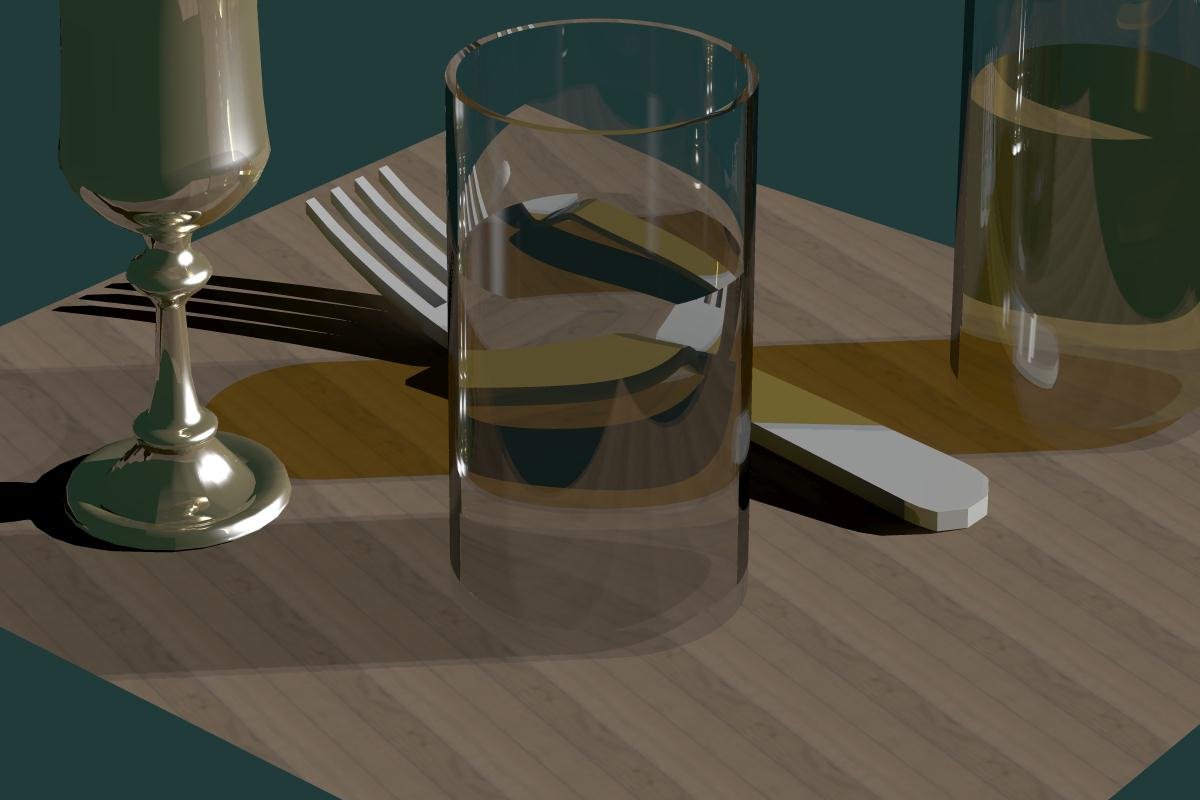
The Monte Carlo algorithm deals with a scene locally: each time a ray-surface intersection is processed the algorithm needs surface properties only in the intersection point. On the other hand, the deterministic algorithm adopts the radiosity scheme, it considers all triangles as a whole. As a result, it has very limited possibilities to account for surface properties variation inside a triangle. These variations may include: surface normal change (in case of curved surfaces); surface color (or an optical parameter) variation (in case of a textured object). In practice it means that the deterministic algorithm can produce a noticeable error if textures are used in a scene or a scene contains curved specularly reflecting surfaces. Also, as was mentioned in the previous chapter, the deterministic algorithm does not account for light refraction (Figure 1a).
|
|
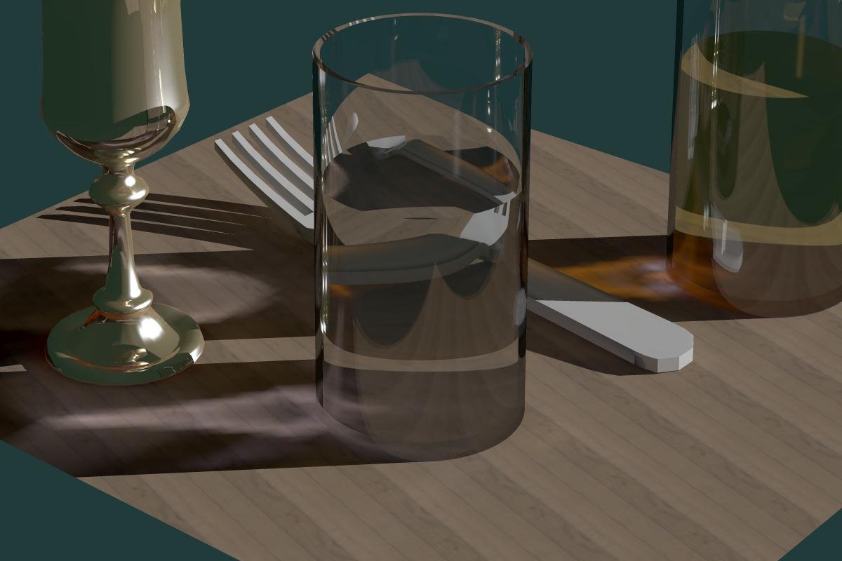
| (a) by Deterministic algorithm | (b) by Monte Carlo algorithm |
| (1024x768 98K) | (1024x768 98K) |
Figure 1. Illumination through refractive objects
The Monte Carlo algorithm correctly accounts for all mentioned phenomena (compare Fig. 1a and Fig. 1b). It means that we should make some precautions to avoid certainly false results of the deterministic algorithm. In practice, we did the following:
(1) Switched off textures if they were used in scenes.
(2) Didn't use for comparison scenes that contained curved mirrors or transparent refractive objects.
All scenes used in the comparison satisfy to the above restrictions.
On the other hand there exist scenes where the deterministic algorithm can produce better results than the Monte Carlo algorithm. These are scenes with plane (specularly) reflective surfaces. Illumination by light reflected by such surfaces is accounted in the deterministic algorithm with use of "virtual source" method while the Monte Carlo algorithm treats this light in its general scheme, as a secondary illumination. This may lead to a better accuracy of this illumination distribution in the Deterministic algorithm. See some more details in ch. Results obtained when particular images are discussed.
|
|
Contents Introduction Overview of Deterministic algorithm Overview of Monte Carlo algorithm Scenes used for comparison Accuracy analysis Results obtained Conclusion Acknowledgments |
|
|
|
|
| Copyright 1996 Andrei Khodulev. | [Home] |