|
Tracking the Trajectories of Evolution
Mikhail S. Burtsev
Address: Keldysh Institute of Applied Mathematics, 4 Miusskaya sq., Moscow RU-125047, Russia E-mail: mbur@narod.ru URL: http://www.keldysh.ru/pages/mrbur-web/
Abstract
This paper proposes a method of visualizing and measuring evolution in Artificial Life simulations. The evolving population of agents is treated as a dynamical system. The proposed method is inspired by the notion of trajectory. This paper provides examples of tracking of trajectories of evolutionary system in the spaces of genotypes, strategies and some global characteristics. Visualization similar to bifurcation diagram is used to represent results of series of simulations.
Keywords: artificial life, evolution, dynamical system, trajectory Introduction
A computer model is a dream of scientist. One can easily measure any aspect of phenomenon observed in simulation. Everything in computer model is measurable. This is a great problem in studying phenomena emerged in computer experiments. One can measure everything, but how to choose features relevant to the problem under consideration? And, how do one need to represent raw data to catch interesting characteristics of the model?
We could found only what we are looking for; our hypotheses about modeled phenomenon guide our choice of features to track in simulations. The main assumptions underling an evolutionary ALife simulations are variation and selection. The questions in this case are what and how selected, and how features of variation affects selection.
The largest part of measures of selection in the field of ALife is based on the notion of fitness. Usually fitness is introduced by authors as function of some features of the evolving component of the model, and this function is expected to estimate "success" in surviving somehow. In the field of engineering applications of evolutionary computations, fitness is introduced explicitly and reflects goals of designer. But in evolutionary biology and Artificial Life using of fitness is controversial, and in every particular circumstance it should be clearly stated what the fitness is and why it is expected to reflect survivability. There are a few popular definitions of fitness in ALife community such as, rate of replication, population size or amount of resources extracted by agents from environment.
The fitness assignment leads to the notion of "fitness landscape". This notion probably is the most widely used in the fields of ALife and evolutionary computations. There are numerous attempts to plot fitness landscapes and how they change [4,10-12,22]. Visualization of fitness landscapes is not an easy task. First of all these landscapes usually have high dimension, and additional information and algorithms needed to project landscape on the plane of low dimension without loss of meaningful traits. The second problem with fitness landscapes is that calculation of such landscapes is usually costly computational. Typically one visualizes a track of a model on a fitness landscape which was produced during simulation, and not the every point in the some region of interest on the landscape.
Another way to deal with selection is to measure persistence of evolving components during the run. It looks like, that we assign to all components of evolving system existed at the moment equal fitness. This means, that if the component exists at the moment, it is fit to the environment. The well-known measure of this kind is an evolutionary activity statistics proposed by Bedau and Packard [5,7,20]. Activity statistics evaluate integral persistence of the component in the course of simulation. The evolutionary activity statistics were successfully used for visualization in a number of studies [6,8,15].
One more approach to look inside ALife simulation is recording pedigree relations, emerged during the run, and then visualizing them as ancestor-descendent graph or diagram [3,23]. This kind of visualization provides clear picture of evolutionary history. Unfortunately, simulations may generate very complicated pedigree relations, in these cases additional tools of analyses are needed.
An alternative view on evolving systems could be offered by dynamical systems theory. A lot of work in this direction has been done in the area of GA [14,17-19,24,25], where the population of solutions was treated as a dynamical system, but little has been done in the field of artificial life.
Dynamical systems theory studies movement of a system. One of the main notions in this theory is the notion of trajectory. It may be the trajectory of the whole system in space, or trajectories of constituted parts in some phase space. Stability, cycles and branching of trajectory could be studied. This paper is an attempt to apply the metaphor of system movement along trajectory in the study of Artificial Life model.
The following section provides a description of the ALife model, and the subsequent section presents the analyses of evolutionary system dynamics for a particular simulation.
The Model
The model belongs to a set of classic ALife models [1,16,21,26] with simple agents and a simple world. The presented implementation of the model was developed to study the evolution of kin-selection, but is used here to demonstrate a results of application of dynamical systems approach to the analyses of the model.
The world in the model is a two dimensional grid, which is closed to form a torus. There are agents and grass in the world. Only one patch of grass can exist in any cell at a given moment of time, but the number of agents in any cell is unlimited. Patches of grass appears randomly at the constant rate and are uniformly distributed in the space.
An agent can observe its local environment and perform certain actions. The agent is oriented in space and has a field of vision. The field of vision consists of four cells: the cell the agent currently occupies, and the adjacent cells directly to the left, front, and right relative to the orientation of the agent. The agent lives in a discrete time. The agent executes one of seven actions during the one time step: to rest, to eat, to turn to the left/right, to move forward to the next cell, to divide, or to fight.
When the agent rests, it changes nothing in the environment. If there is a grass patch in the cell with an agent and it executes the "eat" action, the patch disappears. If the agent divides, an offspring is created and placed in the cell. The agent might also “fight” a randomly chosen agent in the cell.
Each agent stores a finite amount of energy on which to live. When the agent performs any action, its energy resource decreases. If the agent executes the action "to eat" and there is grass in the cell, the energy resource of the agent increases. When the agent produces offspring, the parent spends some amount energy in the process and gives half of the rest to the newborn. After executing of "fight" action, the agent takes some amount of energy from the victim. If the internal energy resource goes to zero, the agent dies.
Behavior of the agent is governed by a simple control system, in which each output, associated with certain action, is connected with each input, associated with certain sensory input from environment or internal state of the agent. The control system is a linear system, which is functioning similar to a feedforward neural network with no hidden layer. To calculate the output vector O of values, the input vector I should be multiplied by a matrix of weights W. Values of W are integers in the range [‑Wmax,Wmax].
At each time step, the agent performs the action associated with the maximum output value.
The input vector I is filled with information about presence of food and other agents in the field of vision, level of internal energy and kinship of randomly chosen agent in the cell, where the agent is situated. The kinship is calculated as Euclidean distance between "kinship marker" vectors of agents.
The weights of the control system are coded in the genome of the agent.
The genome of the agent S consists of three chromosomes S = (B, W, M). The first chromosome is the bit string which codes the presence or the absence of individual sensory inputs and actions; the second one is the vector of integers which codes the weights of the control system transformation and the third chromosome, also vector of integers, codes the kinship marker of the agent.
If the agent executes the action "divide", an offspring appears. The genome of the offspring is constructed with the aid of the following genetic algorithm:
Additional details of model implementation can be found in Appendix 1.
A case study
The simulation was run with a world of 30 x 30 cells and an initial population of 200. To speed program execution, weights took integer values in the range [-1000,1000] and mutation intensity pw was set to 30. In the simulation, every agent could have no more than 13 sensory inputs and 7 actions, therefore the number of the agent's weights was 91. (Full list of parameters of the simulation is provided in Appendix 2).
If we consider evolving population of agents, we can imagine it as a cloud of points in some space, where position of each point is determined by chosen features of corresponding agent. Below in this paper, terms population and system are synonyms, as are agent and point.
When the system evolves the points will appear and disappear. An obvious measure of any population is its size, and the number of points in the space at the given moment is equal to the population size. The dynamics of population size can provide us with preliminary clues about an evolutionary process. The population size vs. time for the current case study is shown on Fig. 1a. If we omit short transient period in the beginning of the run, the plot could be split on three periods, let's call these periods as "epochs". In our case mean population size during each epoch is almost constant, but has different values for every epoch. The epochs also differ in the character of oscillations. These are signs that points in the cloud emerge and die out during each epoch in specific way, so we can say that dynamical system persists in the different regime during every epoch.
Fig. 1. Population size (a), average generation in the population (b), displacement
of the population centroid in the weights space for the time step
To see how fast points which constitute the system are refreshed, one can trace each agent's generation, i.e. the number of ancestors, and then average it over the population. Change in the average generation in the population over time is presented on Fig. 1b. The graph could be approximated by lines with different slopes inside the different epochs. Therefore, each epoch is characterized by approximately constant rate of generation of new points. The plot makes it clear, that refresh rate during epoch I and III is lower then during epoch II. But on the Fig. 1a population size at epoch II is even lower than at epochs I and III, this leads to conclusion that at epoch II death rate is high and a life time of agents is short.
Above, agents were treated as points, without introduction of particular phase space where these points are located. In the model under consideration, an agent could be represented as point in the space of weights of its control system. There are maximum 91 possible weights for every agent, so the phase space has a dimension of 91.
The rate of
growth of average generation in population multiplied on the mutation intensity
determines upper bound of speed of the system's movement along the trajectory in
the weights space. Higher rates make faster movement possible. To see how the speed
of system's movement changes over the time, one can calculate the centroid of
the population C, by averaging weights over all agents, and then
plotting (Fig. 1c) the Euclidean distance
where i = weight number and N = population size.
This measure reflects the integral displacement of the system in weights space during defined time intervals. The plot shows, that for presented run the speed of the system's movement during epoch II is higher than during epochs I and III. One can conclude that in the second case, the system was situated in a relatively stable state, i.e. attractor, and in the first case undergoes a transition between attractors. This makes it reasonable to interpret epoch II as evolutionary transition. (It should be noticed that the term "evolutionary transition" means here transition between metastable states in evolving system, and should not be confused with widely known term introduced in evolutionary biology by Maynard-Smith and Szathmary[13].)
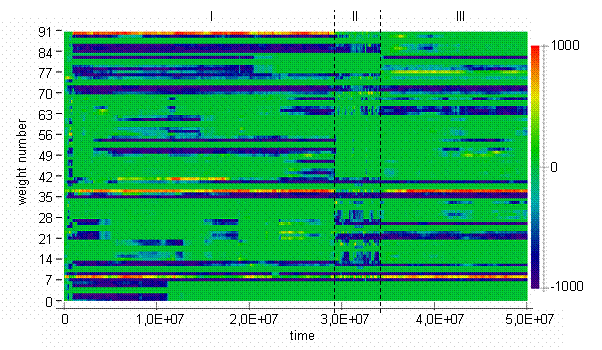
The trajectory of centroid in the weights space can be represented with the aid of a bitmap. Bitmaps are widely used in the fields of ALife and evolutionary computations [2,3,9] for visualization in high dimensional spaces. The bitmap in Fig. 2 reflects the dynamics of the population centroid in the weights space. On the bitmap, weights are grouped by input and it could be seen that incidents of appearance and disappearance of inputs often took place near the edges between epochs. Visualization with a bitmap allows clear separation of values along every dimension in space. On the other hand, it is difficult to compare values on the color scale.
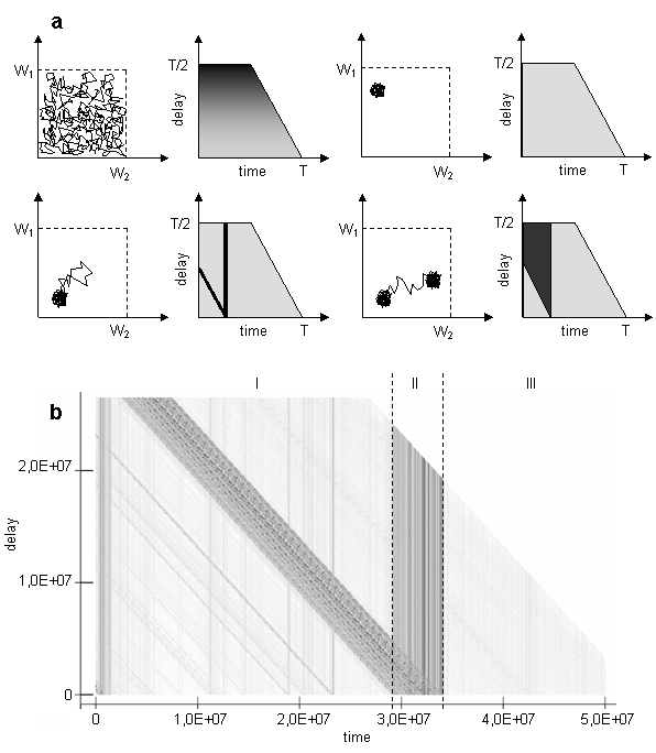
The trajectory of the system can be folded in small region of phase space or continually unfolds; it can also jump between few local regions of attraction or form cycles. To grasp these aspects of trajectory, the bitmap, which consists of horizontal lines, each corresponding to a given delay L (a similar approach was proposed in [9]), can be used (another way of visualizing trajectory was presented in [22]). The level of gray on the Fig. 3 corresponds to the Euclidean distance between the current position of the population centroid and the position after delay:
Such plot can help to identify periodical movement of the centroid over the same points in the phase space, or to determine, if the system has returned to the point, where it was earlier. For example, if there are cycles in the phase space, they should appear as light horizontal bands on the bitmap. Idealized pictures for few basic modes of movement such as random walk, erratic movement around attractor, jump away and return, jump between attractors are provided on the Fig. 3a.
Fig. 2. Centroid weights bitmap [color scale shown on the right]
There are dark vertical lines concentrated inside epoch II on the Figure 3b. When the system is situated in the points corresponded to the vertical dark lines, it is equally far from all subsequent points. On the other hand, dark diagonals represent distance to points at the epoch II from consequent points. So, we can infer that during evolutionary transitions in the model, the population centroid could jump quite far from the areas where it usually persists, and then never return to the points visited during the jump. Other interesting thing about particular run is that relative to the jumps during epoch II trajectory of centroid persists in the same region of weights space at the epoch I as at the epoch III. It is not exactly the same region, if epoch I will be compared to the epoch III (see figure 2). Probably, this region of persistence might be divided on smaller sub-regions as it follows from Figure 2.
Selection in
evolutionary systems acts on the level of behavior of agents, i.e. their
strategies. It is interesting to trace the trajectory of the system in the phase
space of strategies. Usually, a strategies space is relatively large. For the
model under consideration, if we assume that every input can be set to one of
two possible values, the number of possible strategies for 13 inputs and 7
actions can be calculated as
Table 1
Fig. 3. Idealized pictures of distances in phase space for different delays for few basic modes of movement (a) such as random walk, erratic movement around attractor, jump away and return, jump between attractors; diagram for the case study under consideration(b) [on both figures dark is far, light is near]
As a result, strategies space was reduced to 36 = 729 possible strategies. Frequencies of strategies in the population at the given moment of time were calculated by picking every agent and calculating its actions for every situation.
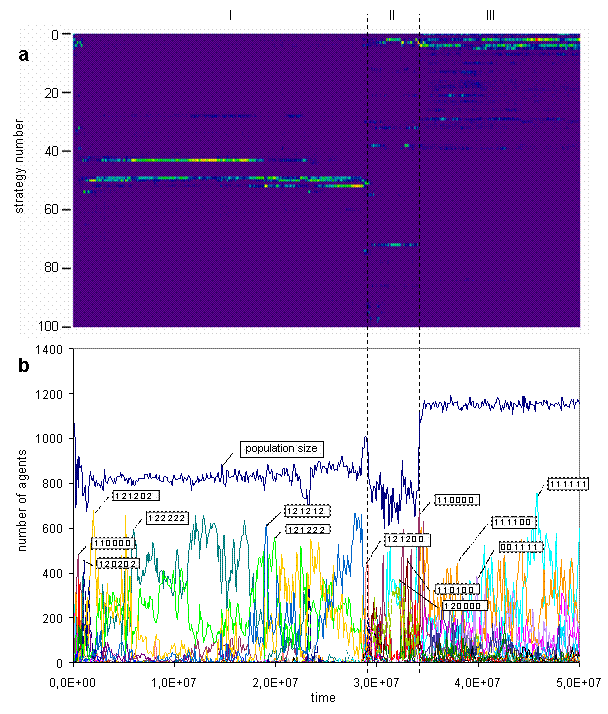
Fig. 4. Strategies bitmap (a) [color scale as on the Fig. 2, but the range starts from 0], strategies graphs (b). (In the simulation discussed here only 142 out of 729 strategies were observed, and frequencies of about one third of them were much smaller than of others, so the bitmap (a) contains only 100 most frequent strategies.)
Actions were grouped by their relevance to the interactions between agents. Table 2
The trajectory of the system in the strategies space is presented on the figure 4. On the Fig. 4a the trajectory visualized as a bitmap and on the Fig. 4b as a set of graphs with callouts. The bitmap better reflects general picture of a strategies dynamics, and graphs offer more detailed representation of main strategies in the population. On the callouts strategies are coded. The numbers refer to the groups of actions and their positions code situation. The even positions are corresponded to kin neighbor, and the odd positions to non kin, internal energy resource is increasing from the left to the right. As seen on the Fig. 4b, during the epoch I kin-selective and aggressive strategies are dominated, then at the epoch II strategies become more peaceful, and at the epoch III the largest part of the population consists of non kin-selective and non aggressive strategies.
The main characteristics for such system of clouds are a number of clouds, weights variance within each cloud and a variance between clouds' centroids. The number of clouds for given case study equals to the number of strategies. Weights variance within cloud could be calculated as:
where N = number of points in the cloud, n = point number, i = weight number, mi = mean value of ith weight in the cloud. And variance between clouds' centroids is defined as:
where Ns = number of strategies in the population, n = strategy number, i = weight number, Cn = centroid for strategy n, C = centroid for strategies' centroids.
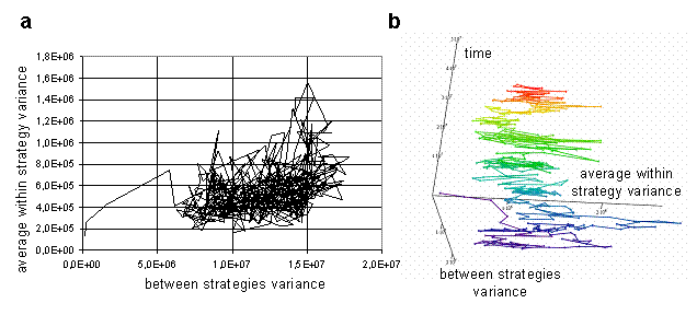
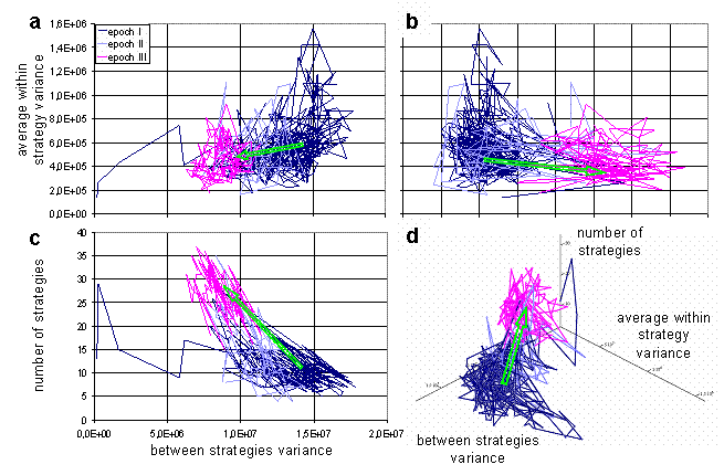
For visualization of dynamics and relations between these characteristics during the run, a phase diagrams can be used. The trajectory of the system in the space of average within and between variances is presented on Fig 5a. The plot provides information about ranges of values of parameters during the run, and also reveals weak correlation between parameters. The higher values of average within strategy variation frequently take place at the high values of between strategies variation. Therefore, when the strategies' clouds in the weight space are close to each other, they are more compact, than when they are far from each over. It is impossible to understand from the plot on Fig. 5a, how trajectory of the system unfolds through the time. To make evolution of system more clear, the plot could be stretched along time axis in the 3d space, as on Fig. 5b. Such stretching offers additional information about changes in the ranges of parameters values through the simulation.
If all three characteristics are plotted by pairs (Fig. 6a,b,c), these graphs forms three projections of 3d image (Fig. 6d). On the Fig. 6 trajectory of the system is marked by different color for each epoch. This marking makes it evident, that the evolutionary system persists in the different regimes during epochs I and III, and undergoes transition between them at the epoch II. During transition the system moves from one area in the characteristics phase space to another. Also, one can see that characteristics on the Fig. 6a and 6b not correlate during every distinct epoch (except fig.6a epoch I, where one can find weak correlation), but there is correlation between characteristics on the Fig. 6c, and the character of this correlation changes from epoch I to epoch III. Figure 6 reveals that during epoch III clouds for strategies in weights space are more compact and closer to each other than during epoch I.
Fig. 5. Average within strategy variance vs. between strategies variance (a), the same plot in 3d space stretched along the time axis (b) [color changes with time].
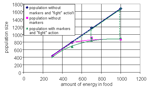
Fig. 6. Three projections: average within strategy variance vs. between strategies variance (a), average within strategy variance vs. number of strategies (b), number of strategies vs. between strategies variance (c); the trajectory in 3d space (d). One particular run is considered above, but normally a series of simulations performed to study behavior of the system for the different parameters. If the dynamics of the system converges to few typical regimes through the series of simulations, then visualization analogous to bifurcation diagram can help us to understand dependence of system's behavior on chosen parameter. Analog of the bifurcation diagram for the presented model is shown on the Fig. 7. On the figure, the size of population in the metastable state is plotted against the amount of energy in the food patch. There are data for three versions of the model. In the first version, agents have no markers and can not fight each other. In the second, agents can fight, but have no markers, and the third is "full" version of the model. Till some amount of energy in the food, steady states for all three systems coincide and population size grows proportional to the energy in the food. Then branching occurs. The line for the first version continues to grow proportional to the energy, when the line for the second freeze on the value, which is equal to the number of cells in the environment. The latter is caused by aggressive behavior of the agents. If two agents are situated in the same cell, they fight each over until one of them will be killed. When markers are added to the model with aggressive agents, there one more metastable state emerges. This state coincides with the one of the first ("peaceful") version. During the runs for the high values of energy in food, the third version of the model first reaches the state similar to the one of the second version. Then, after some period of time, the system "switches" to the state similar to the first version of the model. The simulations expose that switching occurs faster for the higher values of food energy. Such switching is similar to an "avalanches" in self-organized criticality.
Fig. 7. Analog of bifurcation diagram (see text for details).
Discussion
There are two main approaches to the measuring and visualization in the artificial life research. The first one is based on the notion of fitness, and the second is not. Fitness inspired approach emphasizes one or some few of the characteristics of an evolutionary system, and some function of them is treated as measure of survival. In this case, all the other techniques are used to measure and represent dynamics of the selected features and their dependence on the parameters of the model. On the other hand, we don't need fitness, if we want to study evolutionary stable states of the system and transitions between them. So, our viewpoint shifts to measuring and representation of aspects related to stability and change in the system.
In the paper metaphors of dynamical system and its trajectory are used as a source for introduction and interpretation of few ways to measure and visualize ALife simulation. Such approach allows bringing together some existed in the field and a number of new techniques in one coherent framework. Considering population of agents as system one can represent its trajectory in the space of genotypes, phenotypes and in the spaces of different relevant characteristics. Tracking the trajectories of an evolutionary system helps to outline typical regimes or "ways of living" in the system's dynamics, and shed light on their interrelations and origins.
The techniques proposed in the paper have a number of limitations. One limitation is concerned with representing a whole cloud of genotypes in a population as averaged centroid. The parts of the cloud can move intensively, but it will not necessarily cause significant changes in the position of centroid. This problem can be partly resolved by splitting the cloud on parts, each of which will belong to certain phenotype. After partitioning of the cloud, a trajectory of every part's centroid can be tracked independently. Usually, a space of possible phenotypes is large, and one needs to group them somehow. In this paper one of the possible methods is suggested. In this method an experimenter selects a number of situations in the modeled world, and then one picks up every agent in a population and calculates its behavior for every selected circumstances. Afterwards, the agents are grouped in accordance with their behaviors. With no doubt, how to select situations and measure behavior in a particular study remains a hard question, but no any general hints are possible for this problem.
Acknowledgments
Thanks to Gérard Weisbuch for detailed discussion of the first draft of this paper, Yuri Kotov and Frédéric Amblard for comments, Terrill Frantz for proof-reading and style correction. I acknowledge the anonymous reviewers for their suggestions and comments. This work was supported by Russian Fund for Basic Research project # 04-01-00510.
References
Appendix 1: Details of Model Implementation
The agent has storage for internal energy resource R. The capacity of the storage is limited and equals Rmax. When the agent performs actions the resource decreases. If the agent executes action "eat" and there is grass in the cell the energy resource of the agent increases.
The value of internal energy resource of the agent is modified in consistence with the rules summarized in table 3.
Table 3
here ei some constant.
The agent has a marker. The marker m is a vector of length n. Values of components mi are integers in the range [-Mmax,Mmax].
Behavior of the agent is governed by simple control system. This control system has following sensory inputs:
1. Bias. The value of this input is constant and equals k. 2. Four inputs for grass in the field of vision. 3. Number of agents Ni in the cells of the field of
vision. 4. Mean kinship of the cell where the agent is. 5. Information about internal energy resource. 6. Information about similarity between own marker and marker of
neighbor randomly chosen for interaction.
Appendix 2: Parameters of simulation
value description 2 seed of random number generator 30 x size of the world 30 y size of the world 200 initial population size 500000001 number of iterations in simulation 0.005 probability of grass patch appearance in the cell after one time step 700 energy gain of an agent, when it eats a grass patch (Eg) 5000 energy capacity of agent (Rmax) 5 rest energy (e1) 10 turn energy (e2) 20 eat energy (e3) 20 move energy (e4) 20 divide energy (e5) 500 fight energy (e6) 0.001 probability of macromutation (pb) 30 weights mutation intensity (pw) 1000 maximum absolute value of weight (Wmax) 10 dimension of marker vector 100 marker mutation intensity (pm) 1000 maximum absolute value of marker (Mmax)
Every agent in initial population had three sensory inputs and three actions. Weights between these actions are presented in the Table 4. Other actions and sensory inputs were turned off on the chromosome B.
Table 4
|
|||

