Analysis of quasi-steady component in acceleration measurement data obtained onboard Foton M-2
|
|||||||||||||||||||||||||||||||||||||||||||||||||||||||||||||||||||||||||||||||||||||||||||||||||||||||||||||||||||||||||||||||||||||||||||||||||||||||||||||||||||||||||||||||||||||||||||||||||||||||||||||||||||||||||||||||||||||||||||||||||||||||||||||||||||||||||||||||||||||||||||||||||||||||||||||||||||||||||||||||||||||||||||||||||||||||||||||||||||||||||||||||||||||||||||||||||||||||||||||||||||||||||||||||||||||||||||||||||||||||||||||||||||||||||||||||||||||||||||||||||||||||||||||||||||||||||||||||||||||||||||||||||||||||||||||||||||||||||||||||||||||||||||||||||||||||||||||||||||||||||||||||||||||||||||||||||||||||||||||||||||||||||||||||||||||||||||||||||||||||||||||||||||||||||||||||||||||||||||||||||||||||||||||||||||||||||||||||||||||||||||||||||||||||||||||||||||||||||||||||||||||||||||||||||||||||||||||||||||||||||||||||||||||||||||||||||||||||||||||||||||||||||||||||||||||||||||||||||||||||||||||||||||||||||||||||||||||||||||||||||||||||||||||||||||||||||||||||||||||||
 .
.


|
Inter-val |
Date 05/06.2005 |
UTC |
|
deg./s |
deg./s |
deg./s |
deg./s |
|
1 |
31 |
23:25:30 |
2947 |
0.200 |
0.017 |
0.107 |
0.045 |
|
2 |
1 |
11:11:08 |
1318 |
0.312 |
0.014 |
0.082 |
0.045 |
|
3 |
2 |
00:11:50 |
1428 |
0.441 |
0.013 |
0.099 |
0.038 |
|
4 |
2 |
11:12:25 |
1566 |
0.521 |
0.012 |
0.066 |
0.029 |
|
5 |
3 |
00:13:07 |
1038 |
0.645 |
0.016 |
0.070 |
0.024 |
|
6 |
3 |
11:13:43 |
1231 |
0.745 |
0.0070 |
0.056 |
0.016 |
|
7 |
4 |
00:14:24 |
1381 |
0.789 |
0.0059 |
0.094 |
0.029 |
|
8 |
4 |
13:15:06 |
1111 |
0.849 |
0.0067 |
0.145 |
0.013 |
|
9 |
5 |
10:36:15 |
1340 |
0.931 |
0.0059 |
0.147 |
0.011 |
|
10 |
6 |
11:17:34 |
1094 |
1.008 |
0.0072 |
0.146 |
0.011 |
|
11 |
7 |
09:18:45 |
1136 |
1.066 |
0.0039 |
0.131 |
0.0099 |
|
12 |
8 |
09:20:02 |
1210 |
1.111 |
0.0058 |
0.114 |
0.010 |
|
13 |
9 |
09:21:20 |
1147 |
1.149 |
0.0021 |
0.112 |
0.010 |
The table shows
that the angular rate of the satellite increased and formulas (3) became more
precise coupled with this increase (note the behavior of ![]() and
and ![]() ). The final mode of the attitude motion was formed a few
days before the flight termination. There were
). The final mode of the attitude motion was formed a few
days before the flight termination. There were ![]() deg./s and
deg./s and ![]() deg./s [5].
deg./s [5].
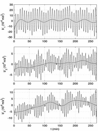
Fig. 2a illustrates
the residual acceleration calculated by formula (1) for the motion in Fig. 1.
Calculations were made for the point ![]() with
with ![]() , where the sensors of the accelerometer TAS3 should be located. The
plots in the figure represent time the components of the vector
, where the sensors of the accelerometer TAS3 should be located. The
plots in the figure represent time the components of the vector ![]() as functions of time.
Here and below, components of vectors are referred to the structural coordinate
system. Calculating the last term in formula (1), we used the ballistic
coefficient obtained by processing trajectory measurements [3]. The atmosphere
density in (1) was calculated according to GOST R (state standard)
25645.166-2004 – Model of the upper atmosphere for ballistic calculations. The
matrices
as functions of time.
Here and below, components of vectors are referred to the structural coordinate
system. Calculating the last term in formula (1), we used the ballistic
coefficient obtained by processing trajectory measurements [3]. The atmosphere
density in (1) was calculated according to GOST R (state standard)
25645.166-2004 – Model of the upper atmosphere for ballistic calculations. The
matrices ![]() of different intervals
of different intervals
![]() somewhat differed from
each other. The acceleration was calculated in each interval
somewhat differed from
each other. The acceleration was calculated in each interval ![]() using the matrix
using the matrix ![]() obtained just for this
interval.
obtained just for this
interval.
3. Filtration of
low-frequency component from TAS3 data. The accelerometer TAS3
measured an apparent acceleration ![]() . Its sensitive axes were parallel to the axes of structural
coordinate system but axes, corresponding to
. Its sensitive axes were parallel to the axes of structural
coordinate system but axes, corresponding to ![]() and
and ![]() , had opposite directions. TAS3 had a sample rate equal to
1000 readings per second and produced the data in a wide spectral range. The
low-frequency filtration of the data was made using finite Fourier series
independently for each vector component.
, had opposite directions. TAS3 had a sample rate equal to
1000 readings per second and produced the data in a wide spectral range. The
low-frequency filtration of the data was made using finite Fourier series
independently for each vector component.
Let ![]() and
and ![]() be natural numbers,
be natural numbers, ![]()
![]() be a segment of the
scalar measurement data. We refer the measurement
be a segment of the
scalar measurement data. We refer the measurement ![]() to the instant
to the instant ![]() ,
, ![]() , and seek the low-frequency component, contained in these
data, in the form
, and seek the low-frequency component, contained in these
data, in the form
 . (4)
. (4)
Here, ![]() are coefficients. They
are found by the least squares method. The simple explicit formulas are
available to calculate them [1]. Some oscillations with relatively high frequencies
are often revealed in function (4) that was obtained in this way. In order to
remove them, some terms in (4) are modified using the correctional multipliers
are coefficients. They
are found by the least squares method. The simple explicit formulas are
available to calculate them [1]. Some oscillations with relatively high frequencies
are often revealed in function (4) that was obtained in this way. In order to
remove them, some terms in (4) are modified using the correctional multipliers

![]() .
.
Here, ![]() is the integer part of
the number
is the integer part of
the number ![]() . As a rule, we don't use expressions (4) directly but deal
with their values
. As a rule, we don't use expressions (4) directly but deal
with their values
![]() ,
, ![]()
![]() ,
, ![]() .
(5)
.
(5)
We refer to these values as
the filtered data. We denote the vector components of the filtered acceleration
data by ![]()
![]() .
.
In all examples
below, expressions (4) were constructed using data segments with a length of
270 min. They were certain of the segments listed in Table 1. The above
procedure was applied at ![]() s,
s, ![]() , and
, and ![]() . The spectrum of functions, obtained in this way, locates
within the limits from 0 to 0.017 Hz. TAS3 measurements have erroneous constant
biases in each vector component. We changed on that reason the coefficient
. The spectrum of functions, obtained in this way, locates
within the limits from 0 to 0.017 Hz. TAS3 measurements have erroneous constant
biases in each vector component. We changed on that reason the coefficient ![]() in (4) to obtain zero
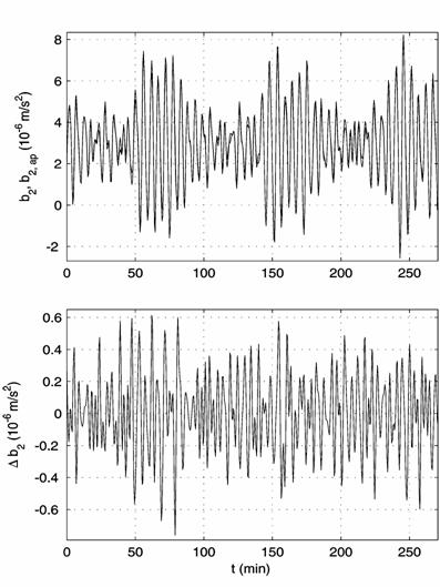
mean value of data (5). Fig. 3a presents the example of the filtered data from
TAS3 measurements. It illustrates the same time interval as Fig. 2a. Each
coordinate system in Fig. 3a contains a couple of plots. The plot of expression
(4) has greater oscillations.
in (4) to obtain zero
mean value of data (5). Fig. 3a presents the example of the filtered data from
TAS3 measurements. It illustrates the same time interval as Fig. 2a. Each
coordinate system in Fig. 3a contains a couple of plots. The plot of expression
(4) has greater oscillations.
TAS3 measurements
contain not only erroneous constant biases but an erroneous infra low-frequency
component too. Such a component has frequencies less than 0.00005 Hz. It is
lacking in calculated accelerations. One should guess it by comparing the plots
in Fig. 3a with the respective plots in Figs. 2a. This effect takes place for
the other intervals of Table 1. To obtain the likeness between the filtered
low-frequency component in TAS3 data and its calculated analog, we eliminated
the infra low-frequency component from data (5). First, we smoothed these data
by the expression
 ,
,
where the coefficients ![]() were found by the
least squares method. We took
were found by the
least squares method. We took ![]() in the case of
in the case of ![]() . The function
. The function ![]() represented the sought
ultra low-frequency component. Then we replaced the quantities
represented the sought
ultra low-frequency component. Then we replaced the quantities ![]() in (5) by the
quantities
in (5) by the
quantities ![]() . Just new data (5) are referred bellow as filtered ones.
These new data are again the values of certain new expression (4).
. Just new data (5) are referred bellow as filtered ones.
These new data are again the values of certain new expression (4).
Fig. 3b presents
the plots of the functions ![]() related to interval
13. Fluent curves in Fig. 3a present the plots of the functions
related to interval
13. Fluent curves in Fig. 3a present the plots of the functions ![]() . When
. When ![]() and
and ![]() , the described method of filtering does not change the
amplitudes of harmonic components in the measurement data with frequencies from
, the described method of filtering does not change the
amplitudes of harmonic components in the measurement data with frequencies from
![]() to
to ![]() Hz; the filtered data
don’t contain harmonics with frequencies higher than
Hz; the filtered data
don’t contain harmonics with frequencies higher than ![]() Hz and lower than
Hz and lower than ![]() Hz.
Hz.
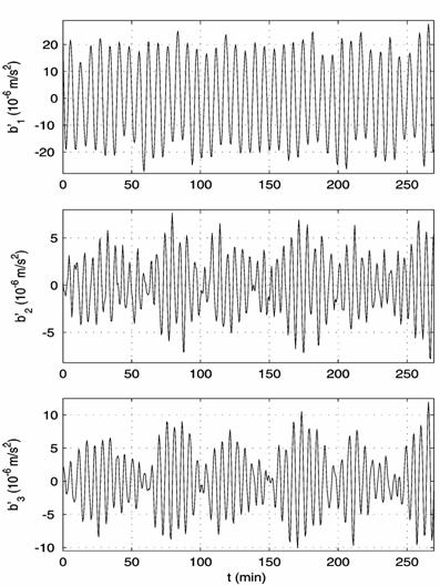
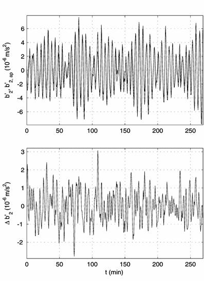
Fig. 2b gives a
comparison of low-frequency component in TAS3 data on interval 13 with its
calculated analog. The plots, drawn by fine lines, were drawn using the
filtered data; the plots, drawn by thick lines, repeat corresponding plots in
Fig. 2a. The thick lines were obtained from the respective lines in Fig. 3b by
the following way. First, we changed the sign of the function ![]() (thereby, we made the
transform
(thereby, we made the
transform ![]() ). Then, we added the constant biases to the functions
). Then, we added the constant biases to the functions ![]() to obtain the
equalities
to obtain the
equalities ![]()
![]() . The operator of mean value
. The operator of mean value ![]() was defined above.
was defined above.
Fig. 2b shows the
functions ![]() and
and ![]() are close. This fact
is valid for intervals 7 – 13 in Table 1. The oscillations of
are close. This fact
is valid for intervals 7 – 13 in Table 1. The oscillations of ![]() and
and ![]() in them have large
amplitudes and frequencies increasing coupled with
in them have large
amplitudes and frequencies increasing coupled with ![]() . It is difficult to see proximity in the case of functions
. It is difficult to see proximity in the case of functions ![]() ,
, ![]() or
or ![]() ,
, ![]() . This is valid for all intervals in Table 1. C. Van Bavinchove, one of
TAS3 creators, supposed the discrepancy was caused of the Earth magnetic field
influence. The next sections contain the analysis confirming this hypothesis.
. This is valid for all intervals in Table 1. C. Van Bavinchove, one of
TAS3 creators, supposed the discrepancy was caused of the Earth magnetic field
influence. The next sections contain the analysis confirming this hypothesis.
4. Spectral
analysis of low-frequency acceleration component. Judging from the plots in
Figs. 2 and 3, the low-frequency component of the acceleration onboard Foton
M-2 can be represented as a linear combination of a few harmonics (cyclic
trends) with frequencies that are incommensurable in the general case. The
representation promises to be especially exact in intervals 7 – 13 in Table 1.
Searching for such harmonics is a typical problem of the time series analysis
[8, 9]. In our case this problem was solved as follows.
Let data (5) be the
filtered data of an acceleration vector component. Expression (4) that
generated them contains harmonics with a fixed set of frequencies. This set has
a formal sense and does not reflect itself spectral properties of the data. In
order to reveal these properties let us try to fit data (5) by the function
![]()
![]() ,
(6)
,
(6)
where ![]() ,
, ![]() ,
, ![]() , and
, and ![]() are parameters. We
will seek the values of these parameters by the least squares method. We make
up the following expression
are parameters. We
will seek the values of these parameters by the least squares method. We make
up the following expression
 (7)
(7)
and minimize it over ![]() ,
, ![]() ,
, ![]() , and
, and ![]() . The function
. The function ![]() has a lot of local
minima and only part of them corresponds to real harmonics. To find such
minima, we solve a number of identical linear least squares problems and calculate
the function
has a lot of local
minima and only part of them corresponds to real harmonics. To find such
minima, we solve a number of identical linear least squares problems and calculate
the function
![]()
at points of a sufficiently
fine uniform grid on the interval ![]() . Then the plot of this function is drawn and the approximate
values of minimum points are found. The abscissas of significant (in the value
of
. Then the plot of this function is drawn and the approximate
values of minimum points are found. The abscissas of significant (in the value
of ![]() ) minima are the frequencies of desired harmonics. Let the frequencies
) minima are the frequencies of desired harmonics. Let the frequencies
![]()
![]() be found in this way.
We seek the trend corresponding to them in the form
be found in this way.
We seek the trend corresponding to them in the form
 ,
(8)
,
(8)
where ![]() ,
, ![]() ,
, ![]() , and
, and ![]()
![]() are parameters. The
values of these parameters are found by minimization of the function specified
by relations (7) and (8) using Gauss-Newton's method. This least squares
problem is nonlinear. The initial approximation to its solution is formed by
the frequencies
are parameters. The
values of these parameters are found by minimization of the function specified
by relations (7) and (8) using Gauss-Newton's method. This least squares
problem is nonlinear. The initial approximation to its solution is formed by
the frequencies ![]() and the solution of
the linear least squares problem (7), (8) over
and the solution of
the linear least squares problem (7), (8) over ![]() ,
, ![]() ,
, ![]() with these frequencies.
with these frequencies.
In order to verify
the found solution by simple means, we considered so-called Schuster's
periodogram [6, 7]
 ,
, 
along with the function ![]() . Let data (5) under study be generated by function (8),
where
. Let data (5) under study be generated by function (8),
where ![]() . Then
. Then ![]() , the periodogram has local maxima at points
, the periodogram has local maxima at points ![]() , while
, while ![]()
![]() . Thus, studying the periodogram maxima one can evaluate the
frequencies and amplitudes of harmonic components in data (5).
. Thus, studying the periodogram maxima one can evaluate the
frequencies and amplitudes of harmonic components in data (5).
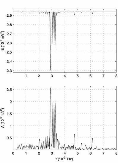
We present below
the plots of the functions
 ,
, ![]()
instead of functions ![]() and
and ![]() . The minima of the function
. The minima of the function ![]() expresses the root
mean square error of approximation of data (5) by sole cyclic trend (6), while
the maxima of function
expresses the root
mean square error of approximation of data (5) by sole cyclic trend (6), while
the maxima of function ![]() estimate the amplitude
estimate the amplitude
![]() .
.
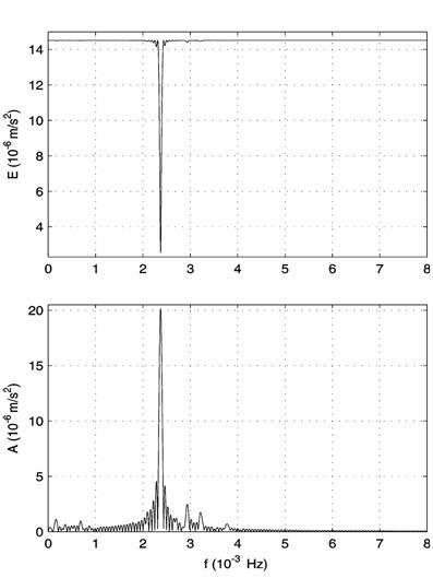
Consider as an
example the results of spectral analysis of the acceleration in Fig. 3b. The
plots of the functions ![]() and
and ![]() for the acceleration
components
for the acceleration
components ![]() and
and ![]() are shown in Figs. 4a,
5a. The component
are shown in Figs. 4a,
5a. The component ![]() has essentially the
same frequency properties as
has essentially the
same frequency properties as ![]() and so it is not
considered in detail. The minimum points of the functions
and so it is not
considered in detail. The minimum points of the functions ![]() differ from the maximum
points of the respective functions
differ from the maximum
points of the respective functions ![]() no more than
no more than ![]() Hz.
Hz.
Each function ![]() or
or ![]() contains several
harmonics. Constructing appropriate expressions (8), we take into account all
clear-cut harmonics (corresponding to well pronounced extrema of
contains several
harmonics. Constructing appropriate expressions (8), we take into account all
clear-cut harmonics (corresponding to well pronounced extrema of ![]() and
and ![]() ) and some of slightly definite ones. To analyze these
expressions, we introduce the following designations. We denote by
) and some of slightly definite ones. To analyze these
expressions, we introduce the following designations. We denote by ![]() expression (8)
approximated the function
expression (8)
approximated the function ![]()
![]() . Plots of the functions
. Plots of the functions ![]() serve to check the approximation.
We refer to the quantity
serve to check the approximation.
We refer to the quantity ![]() as the amplitude of a
harmonic with the frequency
as the amplitude of a
harmonic with the frequency ![]() in (8). The
frequencies and amplitudes of harmonics of
in (8). The
frequencies and amplitudes of harmonics of ![]() are denoted as
are denoted as ![]() and
and ![]() . We also use analogous designations in the case of functions
. We also use analogous designations in the case of functions
![]() and
and ![]() defined in Section 2.
We take
defined in Section 2.
We take ![]() Hz and
Hz and ![]() m/s
m/s![]() as the units for frequencies and acceleration amplitudes
respectively.
as the units for frequencies and acceleration amplitudes
respectively.
The plots of
functions ![]() ,
, ![]() , and
, and ![]() (
(![]() ) are given in Figs. 4b, 5b. We see the approximation is
sufficiently exact. This fact confirms the accuracy of finding the frequencies
) are given in Figs. 4b, 5b. We see the approximation is
sufficiently exact. This fact confirms the accuracy of finding the frequencies ![]() and amplitudes
and amplitudes ![]() that are listed in
Table 2. Here, the frequencies with identical subscripts are approximately
equal and empty cells mean that corresponding harmonics are absent in a respective
function.
that are listed in
Table 2. Here, the frequencies with identical subscripts are approximately
equal and empty cells mean that corresponding harmonics are absent in a respective
function.
Following the least
squares method, we estimate the accuracy of determination of the quantities ![]() and
and ![]() by corresponding
standard deviations. These standard deviations seem to be not adequate from the
probabilistic point of view in this situation but they give useful information.
The frequency
by corresponding
standard deviations. These standard deviations seem to be not adequate from the
probabilistic point of view in this situation but they give useful information.
The frequency ![]() has the least standard
deviation equal to 0.00021; standard deviations of the frequencies
has the least standard
deviation equal to 0.00021; standard deviations of the frequencies ![]() and
and ![]() don’t exceed 0.001;
standard deviations of the other frequencies are within the limits
don’t exceed 0.001;
standard deviations of the other frequencies are within the limits ![]() . Standard deviations of the amplitudes
. Standard deviations of the amplitudes ![]() and
and ![]() don’t exceed 0.3 and
0.15 correspondingly.
don’t exceed 0.3 and
0.15 correspondingly.
The standard
deviations of the frequencies look too small. We point out for comparison that
frequency estimations as minima of ![]() or maxima of
or maxima of ![]() have errors with the
upper bound
have errors with the
upper bound ![]() . We have
. We have ![]() in our case. This
value looks too much great as the accuracy estimate of the frequencies
in our case. This
value looks too much great as the accuracy estimate of the frequencies ![]() .
.
Certain of the
found frequencies admit the obvious interpretation. The frequencies ![]() are caused by
spacecraft orbital motion. The orbital frequency
are caused by
spacecraft orbital motion. The orbital frequency ![]() (the reciprocal
quantity to the orbital period) equals 0.185 so
(the reciprocal
quantity to the orbital period) equals 0.185 so
![]() . (9)
. (9)
Return to formulas (3). The
motion, which they describe, is called the nutational motion and its circular
frequency ![]() is called the nutation
frequency. This circular frequency corresponds to the cyclic frequency
is called the nutation
frequency. This circular frequency corresponds to the cyclic frequency ![]() and we have
and we have ![]() for interval 13. Hence,
for interval 13. Hence,
![]() ,
, ![]() . (10)
. (10)
Just the harmonic with the
greatest amplitude has the frequency ![]() . The spacecraft nutational motion causes it. This result agrees with
formula (1), where the first two terms predominate.
. The spacecraft nutational motion causes it. This result agrees with
formula (1), where the first two terms predominate.
To interpret some
other frequencies, let us assume that the spacecraft performs exact Euler’s
regular precession of an axisymmetric rigid body. Then we have to put ![]() in (3). Euler’s
precession is described usually by the nutation angle
in (3). Euler’s
precession is described usually by the nutation angle ![]() , the precession angle
, the precession angle ![]() and the angle
and the angle ![]() of a proper rotation, the quantities
of a proper rotation, the quantities ![]() ,
, ![]() , and
, and ![]() being constants in the
exact precession. Foton M-2 had [3]
being constants in the
exact precession. Foton M-2 had [3]
 ,
, ![]() ,
, ![]() .
.
A vector that is a constant in
the absolute space has time-dependent components in the system ![]() . These components are sums of constant terms and four harmonics
with the frequencies
. These components are sums of constant terms and four harmonics
with the frequencies
 ,
,  ,
, ![]() ,
, ![]() .
.
The amplitudes of the
harmonics have the order ![]() ,
, ![]() ,
, ![]() , and
, and ![]() respectively when
respectively when ![]() . There are
. There are ![]() ,
, ![]() ,
, ![]() ,
, ![]() in our example. The
harmonic with the frequency
in our example. The
harmonic with the frequency ![]() proved to be
appreciable. We see in Table 2 that
proved to be
appreciable. We see in Table 2 that
Table 2. Frequencies and amplitudes of harmonic components
in the calculated and measured accelerations. Interval 13
|
|
Frequency interpretation |
|
|
|
|
|
|
||||||
|
|
|
|
|
|
|
|
|
|
|
|
|
||
|
1 |
|
|
|
|
|
|
|
0.158 |
0.983 |
|
|
|
|
|
2 |
|
0.371 |
2.011 |
|
|
0.367 |
0.531 |
|
|
|
|
|
|
|
3 |
|
0.509 |
1.681 |
|
|
|
|
|
|
|
|
|
|
|
4 |
|
|
|
|
|
|
|
0.698 |
0.699 |
|
|
|
|
|
5 |
|
0.862 |
1.357 |
|
|
|
|
|
|
|
|
|
|
|
6 |
|
|
|
2.044 |
0.478 |
2.035 |
0.600 |
|
|
|
|
|
|
|
7 |
|
|
|
|
|
|
|
|
|
2.215 |
0.214 |
2.215 |
0.173 |
|
8 |
|
2.376 |
20.05 |
|
|
|
|
2.375 |
20.22 |
2.374 |
0.674 |
2.375 |
0.785 |
|
9 |
|
|
|
2.535 |
0.440 |
2.530 |
0.655 |
|
|
2.536 |
0.206 |
2.536 |
0.158 |
|
10 |
|
2.683 |
1.255 |
2.725 |
0.588 |
2.720 |
0.926 |
|
|
2.705 |
0.204 |
2.705 |
0.168 |
|
11 |
|
2.867 |
2.280 |
2.887 |
2.621 |
2.887 |
4.475 |
2.924 |
2.387 |
2.891 |
0.819 |
2.892 |
0.664 |
|
12 |
|
|
|
3.074 |
1.884 |
3.075 |
1.860 |
|
|
3.075 |
2.070 |
3.075 |
1.694 |
|
13 |
|
|
|
3.251 |
2.018 |
3.249 |
2.948 |
3.223 |
1.691 |
3.261 |
0.764 |
3.262 |
0.614 |
|
14 |
|
|
|
|
|
|
|
|
|
3.371 |
0.212 |
3.370 |
0.174 |
|
15 |
|
|
|
|
|
|
|
3.769 |
0.790 |
|
|
|
|
|
16 |
|
|
|
4.746 |
0.632 |
4.750 |
0.606 |
|
|
4.751 |
0.523 |
4.751 |
0.643 |
|
17 |
|
|
|
|
|
|
|
|
|
5.300 |
0.210 |
5.300 |
0.259 |
|
18 |
|
|
|
6.143 |
0.474 |
6.147 |
0.357 |
|
|
6.145 |
0.364 |
6.145 |
0.447 |
![]() .
(11)
.
(11)
We see also that
![]() ,
, ![]() . (12)
. (12)
The harmonics with the
frequencies ![]() ,
, ![]() , and
, and ![]() can be explained by
the last two terms in formula (1). In particular, the components of the last
term that describes the atmosphere drag are presented in the geocentric absolute
coordinate system by periodical functions with the orbital period. The second
column in Table 2 summarizes our interpretation of some found frequencies.
can be explained by
the last two terms in formula (1). In particular, the components of the last
term that describes the atmosphere drag are presented in the geocentric absolute
coordinate system by periodical functions with the orbital period. The second
column in Table 2 summarizes our interpretation of some found frequencies.
We performed in the
same way the spectral analysis of the functions ![]() plotted in Fig. 2a. Its results are presented in Tables 2 and
Figs. 6, 7. We omitted plots relating to the function
plotted in Fig. 2a. Its results are presented in Tables 2 and
Figs. 6, 7. We omitted plots relating to the function ![]() because it has the
same frequency properties as
because it has the
same frequency properties as ![]() . Accuracy characteristics of the found harmonics are
following. The frequency
. Accuracy characteristics of the found harmonics are
following. The frequency ![]() has the least standard
deviation equal to 0.00011; standard deviations of the frequencies
has the least standard
deviation equal to 0.00011; standard deviations of the frequencies ![]() and
and ![]()
![]() don’t exceed 0.001;
standard deviations of the other frequencies are within the limits
don’t exceed 0.001;
standard deviations of the other frequencies are within the limits ![]() . Standard deviations of the amplitudes
. Standard deviations of the amplitudes ![]() and
and ![]() don’t exceed 0.14 and
0.04 respectively.
don’t exceed 0.14 and
0.04 respectively.
One can see from
Table 2 that the functions ![]() contain harmonics with
about the same frequencies as the functions
contain harmonics with
about the same frequencies as the functions ![]() . Therefore we used the same principle of the frequency numbering.
The close frequencies are in the same line in Table 2. It is not surprising
that the frequencies of functions
. Therefore we used the same principle of the frequency numbering.
The close frequencies are in the same line in Table 2. It is not surprising
that the frequencies of functions ![]() satisfy the relations
(9) – (12). However amplitudes of some corresponding harmonics in
satisfy the relations
(9) – (12). However amplitudes of some corresponding harmonics in ![]() and
and ![]() differ markedly. The
greatest discrepancy of amplitudes takes place for harmonics with the
frequencies
differ markedly. The
greatest discrepancy of amplitudes takes place for harmonics with the
frequencies ![]() and
and ![]() . There is only one good coincidence of amplitudes. It takes
place for harmonics with the frequency
. There is only one good coincidence of amplitudes. It takes
place for harmonics with the frequency ![]() . We see some coincidence in the case of frequencies
. We see some coincidence in the case of frequencies ![]() . Some discrepancy in the case of frequencies
. Some discrepancy in the case of frequencies ![]() and
and ![]() can be explained by
our pared-down using the TAS3 geometrical characteristics. The single-axis
sensors for different directions had slightly different coordinates in this
device whereas we use the same coordinates for each sensor.
can be explained by
our pared-down using the TAS3 geometrical characteristics. The single-axis
sensors for different directions had slightly different coordinates in this
device whereas we use the same coordinates for each sensor.
It is worth to note
that the discrepancy between corresponding frequencies of functions ![]() and
and ![]() are distinctly smaller
than errors in their interpretation in terms of
are distinctly smaller
than errors in their interpretation in terms of ![]() ,
, ![]() and
and ![]() . Possibly, the inaccuracy of the interpretation is caused by
some fine details of the motion.
. Possibly, the inaccuracy of the interpretation is caused by
some fine details of the motion.
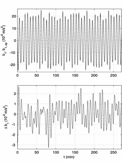
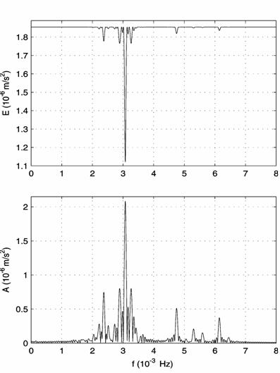
Now, we turn to the
spectral analysis of the components of the magnetic field strength. We
investigated the functions ![]() calculated by formulas
(2) and plotted in Fig. 1a. The investigation of the functions
calculated by formulas
(2) and plotted in Fig. 1a. The investigation of the functions ![]() gave the same results.
The analysis was made according to the scheme above. Its results are presented
in Table 3 and Figs. 8, 9. The table and figures are arranged in the same
manner as Table 2 and Figs. 4 – 7. The functions
gave the same results.
The analysis was made according to the scheme above. Its results are presented
in Table 3 and Figs. 8, 9. The table and figures are arranged in the same
manner as Table 2 and Figs. 4 – 7. The functions ![]() and
and ![]() have the same frequency
properties, so we cited the plots for
have the same frequency
properties, so we cited the plots for ![]() only. The quantities
only. The quantities ![]() and
and ![]() in Table 3 have the
standard deviations equal to 0.0062 and 7000
in Table 3 have the
standard deviations equal to 0.0062 and 7000![]() respectively. The frequencies
respectively. The frequencies ![]() and
and ![]() have the least
standard deviations equal to 0.00019; standard deviations of the frequencies
have the least
standard deviations equal to 0.00019; standard deviations of the frequencies ![]() and
and ![]() don’t exceed 0.0004;
standard deviations of the other frequencies are within the limits
don’t exceed 0.0004;
standard deviations of the other frequencies are within the limits ![]() . Standard deviations of the amplitudes
. Standard deviations of the amplitudes ![]() , except
, except ![]() , don’t exceed 300
, don’t exceed 300![]() .
.
The functions ![]() contain some harmonics
with about the same frequencies as the functions
contain some harmonics
with about the same frequencies as the functions ![]() and
and ![]() . The first column of Table 3 gives in brackets the number of
a close frequency from Table 2. Therefore it was not surprising that some
frequencies, found in the functions
. The first column of Table 3 gives in brackets the number of
a close frequency from Table 2. Therefore it was not surprising that some
frequencies, found in the functions ![]() , admit the obvious interpretation. Namely, we have the
relations
, admit the obvious interpretation. Namely, we have the
relations
![]() ,
, ![]() ,
, ![]() ,
, ![]()
for frequencies of harmonics
with large amplitudes and we have the relations
![]() ,
, ![]()
for frequencies of harmonics
with small amplitudes.
The frequencies ![]() and
and ![]() appear both in the functions
appear both in the functions ![]() and in the functions
and in the functions ![]() . But their presence in
. But their presence in ![]() is much more greater –
the corresponding harmonics have much more greater amplitudes. It is worth to
compare this fact with the following one. The frequency
is much more greater –
the corresponding harmonics have much more greater amplitudes. It is worth to
compare this fact with the following one. The frequency ![]() is present in
functions
is present in
functions ![]() and
and ![]() too; the amplitudes of
corresponding harmonics are approximately equal in all these functions and are
twice greater than amplitudes of harmonics with frequencies
too; the amplitudes of
corresponding harmonics are approximately equal in all these functions and are
twice greater than amplitudes of harmonics with frequencies ![]() ,
, ![]() in
in ![]() . Thus transition
. Thus transition ![]() doesn't change the
amplitudes for the frequency
doesn't change the
amplitudes for the frequency ![]() , which is absent in the functions
, which is absent in the functions ![]() , and essentially increases the amplitudes for the
frequencies
, and essentially increases the amplitudes for the
frequencies ![]() ,
, ![]() , which are present in the functions
, which are present in the functions ![]() . This situation is illustrated by comparison of Figs. 5a,
7a, and 9a. The comparison shows that the function
. This situation is illustrated by comparison of Figs. 5a,
7a, and 9a. The comparison shows that the function ![]() inherits the
frequencies from the functions
inherits the
frequencies from the functions ![]() and
and ![]() . The same inheritance takes place in the case of functions
. The same inheritance takes place in the case of functions ![]() ,
, ![]() and
and ![]() (compare corresponding
columns in Tables 2, 3). The analogous inheritance in the case of functions
(compare corresponding
columns in Tables 2, 3). The analogous inheritance in the case of functions ![]() ,
, ![]() , and
, and ![]() is not so pronounced
(see Figs. 4a, 6a, and 8a) against a background of the large amplitudes of the
harmonics with the frequency
is not so pronounced
(see Figs. 4a, 6a, and 8a) against a background of the large amplitudes of the
harmonics with the frequency ![]() in
in ![]() and
and ![]() . But if we calculate amplitude ratios for harmonics with
frequencies closed to
. But if we calculate amplitude ratios for harmonics with
frequencies closed to ![]() in
in ![]() and
and ![]() , we find the influence of the magnetic field has here the
same order as in the case of the functions
, we find the influence of the magnetic field has here the
same order as in the case of the functions ![]() and
and ![]() . Quantitative characteristics of the influence will be
described below.
. Quantitative characteristics of the influence will be
described below.
Table
3. Frequencies and amplitudes of harmonic
components
in the magnetic field strength.
|
|
Frequency interpretation |
|
|
|
|||
|
|
|
|
|
|
|
||
|
1 |
|
0.026 |
13960 |
|
|
|
|
|
2(1) |
|
0.193 |
3297 |
|
|
|
|
|
3(2) |
|
0.339 |
20240 |
|
|
|
|
|
4(3) |
|
0.510 |
13164 |
|
|
|
|
|
5(4) |
|
0.700 |
1775 |
|
|
|
|
|
6(5) |
|
0.868 |
6032 |
|
|
|
|
|
7(6) |
|
|
|
2.039 |
3697 |
2.039 |
3707 |
|
8(8) |
|
|
|
2.365 |
3362 |
2.364 |
3394 |
|
9(9) |
|
|
|
2.526 |
3892 |
2.526 |
3851 |
|
10(10) |
|
|
|
2.717 |
5831 |
2.717 |
5849 |
|
11(11) |
|
|
|
2.887 |
28042 |
2.887 |
28067 |
|
12(13) |
|
|
|
3.245 |
14010 |
3.245 |
14011 |
|
13 |
|
|
|
3.433 |
1648 |
3.433 |
1671 |
|
14 |
|
|
|
3.566 |
2790 |
3.566 |
2770 |
The analogous
analysis was made for interval 9 from Table 1 to investigate the influence of
variations of ![]() on the results
obtained. New results proved to be in a good agreement with the previous ones.
We have
on the results
obtained. New results proved to be in a good agreement with the previous ones.
We have ![]() and
and ![]() based on
based on ![]() for interval 9. The
transition
for interval 9. The
transition ![]() increases the
amplitudes for frequencies
increases the
amplitudes for frequencies ![]() and
and ![]() which are present in the
functions
which are present in the
functions ![]() . The transition
. The transition ![]() increases the
amplitude for frequency
increases the
amplitude for frequency ![]() , which is present in the function
, which is present in the function ![]() .
.
5. Correction of
filtered TAS3 measurement data. As long as the main frequencies of the
functions ![]() are obtained by joining
up the main frequencies of the functions
are obtained by joining
up the main frequencies of the functions ![]() and
and ![]() , we can assume that the Earth magnetic field influenced upon
TAS3 measurements linearly. This assumption gives hope to us that TAS3 filtered
data can be corrected by the formulas
, we can assume that the Earth magnetic field influenced upon
TAS3 measurements linearly. This assumption gives hope to us that TAS3 filtered
data can be corrected by the formulas

![]() ,
,
where ![]() are constants. We
suppose here and below in this Section that the sign of the component
are constants. We
suppose here and below in this Section that the sign of the component ![]() has been changed.
has been changed.
If we make a
correction for the magnetic field, it is naturally to make simultaneously some
other corrections, namely, the correction for infra low-frequency errors, the
correction for the shift of TAS3 time scale, the correction for the error in
the spacecraft ballistic coefficient and the correction for misalignment of
sensitive TAS3 axes with respect to the axes ![]() . We specify the last correction by the vector
. We specify the last correction by the vector ![]() of infinitesimal
rotation of TAS3 sensitive axes with respect to the system
of infinitesimal
rotation of TAS3 sensitive axes with respect to the system ![]() . The components of
. The components of ![]() can be regarded both
to the system
can be regarded both
to the system ![]() and to the system
formed by sensitive axes of TAS3. The correction of the ballistic coefficient
is specified by means of multiplication of it by the factor
and to the system
formed by sensitive axes of TAS3. The correction of the ballistic coefficient
is specified by means of multiplication of it by the factor ![]() :
: ![]() . This correction compensates short time variations of
. This correction compensates short time variations of ![]() and
and ![]() within a long interval
in which
within a long interval
in which ![]() was defined. Taking
into account all these corrections and assuming they allow removing all
possible errors, we can write
was defined. Taking
into account all these corrections and assuming they allow removing all
possible errors, we can write

 ,
,
 (13)
(13)
 ,
,

 ,
,

![]() .
.
Here, the functions ![]() compensate infra
low-frequency errors in filtered data,
compensate infra
low-frequency errors in filtered data, ![]() is the shift of TAS3
time scale with respect to the time scale used for description of spacecraft
attitude motion, the functions
is the shift of TAS3
time scale with respect to the time scale used for description of spacecraft
attitude motion, the functions ![]() and
and ![]() are defined by
relations (see (1),
are defined by
relations (see (1), ![]() are unit vectors along
the axes
are unit vectors along
the axes ![]() )
)
 ,
,  ,
,
the quantities ![]() set the origin of TAS3
coordinate system with respect to the spacecraft mass center,
set the origin of TAS3
coordinate system with respect to the spacecraft mass center, ![]()
![]() are the coordinates of
the TAS3 sensor for
are the coordinates of
the TAS3 sensor for
the axis ![]() in the TAS3 own coordinate
system,
in the TAS3 own coordinate
system,
![]() mm,
mm, ![]() mm,
mm, ![]() mm,
mm,
![]() mm,
mm, ![]() mm,
mm, ![]() mm,
mm,
![]() mm,
mm, ![]() mm,
mm, ![]() mm,
mm,
We considered
relations (13) as equations for determining the unknown quantities ![]() ,
, ![]() ,
, ![]() ,
, ![]() ,
, ![]() , and
, and ![]() . We look for these quantities in the following way. Let
. We look for these quantities in the following way. Let ![]() be given. We consider
relations (13) at the points
be given. We consider
relations (13) at the points ![]() defined by formulas
(5). The quantities
defined by formulas
(5). The quantities ![]() are calculated at
filtration and we don’t exclude the infra low-frequency component from them
because this corrections are provided by functions
are calculated at
filtration and we don’t exclude the infra low-frequency component from them
because this corrections are provided by functions ![]() . The quantities
. The quantities ![]() and
and ![]() are calculated by
interpolation using finite Fourier series. Those series were constructed beforehand
basing on the proper solution of spacecraft motion equations. We obtained as a
result the overdetermined linear system with the unknown quantities
are calculated by
interpolation using finite Fourier series. Those series were constructed beforehand
basing on the proper solution of spacecraft motion equations. We obtained as a
result the overdetermined linear system with the unknown quantities ![]() ,
, ![]() ,
, ![]() ,
, ![]() , and
, and ![]() . We treat the problem of finding its solution as a standard
linear regression problem. We solve it by the least squares method for each
. We treat the problem of finding its solution as a standard
linear regression problem. We solve it by the least squares method for each ![]() at points of the uniform
grid with the step 1 s and calculate the standard deviation
at points of the uniform
grid with the step 1 s and calculate the standard deviation ![]() of discrepancies in
(13). The value
of discrepancies in
(13). The value ![]() is considered to be
the required estimate of
is considered to be
the required estimate of ![]() . The solution of the regression problem at
. The solution of the regression problem at ![]() gives us the required
estimates of the quantities listed above. The standard deviations of those quantities,
calculated at
gives us the required
estimates of the quantities listed above. The standard deviations of those quantities,
calculated at ![]() in the framework of a
linear regression problem previously mentioned, are adopted as accuracy
characteristics of the found estimates. We emphasize the standard deviations are
calculated at fixed
in the framework of a
linear regression problem previously mentioned, are adopted as accuracy
characteristics of the found estimates. We emphasize the standard deviations are
calculated at fixed ![]() , which is supposed to be known, and are so-called
conditional standard deviations. The unconditional standard deviation
, which is supposed to be known, and are so-called
conditional standard deviations. The unconditional standard deviation ![]() of the estimate
of the estimate ![]() is calculated by the
formula
is calculated by the
formula
 .
.
The results of
solution of the regression problem are presented in Table 4 and Figs. 10 – 12.
These results were obtained for some intervals from Table 1. They were obtained
at ![]() but they almost
coincide with the results for
but they almost
coincide with the results for ![]() and
and ![]() . Table 4 contains the estimates of the quantities
. Table 4 contains the estimates of the quantities ![]() ,
, ![]() ,
, ![]() ,
, ![]() , and
, and ![]() as well as their
standard deviations. The unit of
as well as their
standard deviations. The unit of ![]() and
and ![]() is radian, the unit of
is radian, the unit of
![]() and
and ![]() is
is ![]() m/(s
m/(s![]() Oe).
Oe).
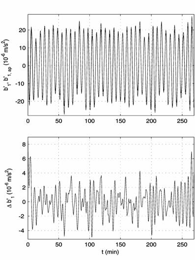
Figs. 10a, 11a, and
12a contain the plots of the functions ![]() and
and ![]()
![]() defined by the
left-hand sides and right-hand sides of formulas (13). Thick lines depict the
plots of the functions
defined by the
left-hand sides and right-hand sides of formulas (13). Thick lines depict the
plots of the functions ![]() ; fine lines depict the plots of the
; fine lines depict the plots of the
Table 4. Estimations of TAS3
adjusting parameters. The unit of ![]() and
and ![]() is
is ![]() m/(s
m/(s![]() Oe)
Oe)
|
Interval |
|
s |
s |
mm |
mm |
mm |
mm |
mm |
mm |
|
|
|
1 |
0.764 |
–48 |
3.0 |
22.3 |
19 |
–121.0 |
5.5 |
–219.8 |
4.5 |
0.929 |
0.023 |
|
2 |
0.675 |
–37 |
2.4 |
–13.7 |
13 |
–96.9 |
2.9 |
–229.1 |
2.8 |
1.089 |
0.016 |
|
4 |
0.801 |
–22 |
2.5 |
–16.7 |
13 |
–109.8 |
2.5 |
–231.0 |
2.4 |
1.179 |
0.020 |
|
6 |
0.748 |
–32 |
1.7 |
1.6 |
12 |
–86.0 |
1.9 |
–227.2 |
1.9 |
1.043 |
0.020 |
|
8 |
0.781 |
–25 |
1.7 |
–7.0 |
5.0 |
–94.3 |
0.74 |
–241.2 |
0.73 |
1.095 |
0.015 |
|
9 |
0.999 |
–32 |
1.8 |
–8.1 |
5.8 |
–63.6 |
0.83 |
–238.8 |
0.82 |
0.939 |
0.016 |
|
10 |
0.742 |
–23 |
1.2 |
–8.4 |
4.1 |
–96.1 |
0.57 |
–235.8 |
0.57 |
0.900 |
0.012 |
|
11 |
0.745 |
–19 |
1.4 |
–10.9 |
4.3 |
–96.8 |
0.60 |
–226.1 |
0.60 |
1.078 |
0.013 |
|
12 |
0.952 |
–23 |
1.9 |
–9.8 |
6.0 |
–69.4 |
0.85 |
–236.4 |
0.84 |
0.895 |
0.017 |
|
13 |
0.734 |
–15 |
1.2 |
–7.8 |
4.6 |
–104.2 |
0.66 |
–229.8 |
0.64 |
1.040 |
0.014 |
|
Interval |
|
|
|
|
|
|
|
|
|
|
|
|
|
1 |
0.002 |
0.020 |
–0.039 |
0.017 |
0.0007 |
0.013 |
–189.2 |
2.9 |
–5.1 |
2.1 |
–87.2 |
3.5 |
|
2 |
0.040 |
0.013 |
0.014 |
0.011 |
0.020 |
0.0085 |
–197.9 |
1.9 |
–16.6 |
1.9 |
–101.8 |
2.3 |
|
4 |
–0.099 |
0.016 |
–0.010 |
0.0099 |
0.006 |
0.0076 |
–184.6 |
1.7 |
–15.8 |
1.9 |
–97.2 |
2.4 |
|
6 |
0.060 |
0.015 |
–0.017 |
0.0089 |
0.040 |
0.0064 |
–191.0 |
1.6 |
–5.3 |
1.7 |
–99.5 |
2.2 |
|
8 |
–0.008 |
0.012 |
–0.034 |
0.0037 |
0.026 |
0.0025 |
–186.9 |
2.8 |
–16.7 |
1.4 |
–98.2 |
1.5 |
|
9 |
0.132 |
0.014 |
–0.010 |
0.0043 |
0.018 |
0.0028 |
–188.7 |
2.9 |
–1.8 |
1.9 |
–105.2 |
2.0 |
|
10 |
–0.026 |
0.011 |
–0.033 |
0.0030 |
0.024 |
0.0019 |
–189.0 |
2.5 |
–14.9 |
1.4 |
–100.8 |
1.5 |
|
11 |
0.022 |
0.011 |
–0.026 |
0.0032 |
0.012 |
0.0021 |
–178.8 |
3.0 |
–13.5 |
1.4 |
–96.4 |
1.5 |
|
12 |
0.161 |
0.015 |
–0.021 |
0.0044 |
0.022 |
0.0029 |
–185.9 |
3.1 |
–6.6 |
1.9 |
–101.8 |
2.0 |
|
13 |
–0.043 |
0.013 |
–0.040 |
0.0034 |
0.013 |
0.0022 |
–184.1 |
2.6 |
–18.1 |
1.4 |
–99.6 |
1.5 |
Table 4 (continuation).
Estimations of TAS3 adjusting parameters. The unit of ![]() and
and ![]() is
is ![]() m/(s
m/(s![]() Oe)
Oe)
|
Interval |
|
|
|
|
|
|
|
|
|
|
|
|
|
1 |
6.6 |
3.2 |
–104.4 |
1.6 |
–26.7 |
3.9 |
–21.9 |
3.6 |
–1.9 |
2.3 |
–169.4 |
2.8 |
|
2 |
3.1 |
2.4 |
–105.9 |
1.7 |
–29.2 |
2.5 |
–14.5 |
2.6 |
–14.5 |
2.0 |
–170.9 |
1.8 |
|
4 |
11.6 |
2.1 |
–111.4 |
1.7 |
–35.2 |
3.2 |
–15.2 |
2.4 |
–10.9 |
2.4 |
–172.0 |
1.8 |
|
6 |
7.8 |
1.9 |
–108.0 |
1.6 |
–26.5 |
3.0 |
–18.3 |
2.2 |
–17.2 |
2.2 |
–176.0 |
1.9 |
|
8 |
2.8 |
2.8 |
–111.7 |
1.5 |
–23.9 |
2.3 |
–11.6 |
2.8 |
–21.7 |
1.8 |
–171.8 |
1.4 |
|
9 |
2.2 |
2.9 |
–98.4 |
1.9 |
–6.8 |
2.9 |
–10.7 |
3.0 |
–9.8 |
2.3 |
–184.8 |
1.9 |
|
10 |
10.3 |
2.5 |
–106.3 |
1.5 |
–26.0 |
2.2 |
–25.4 |
2.6 |
–11.3 |
1.8 |
–174.7 |
1.4 |
|
11 |
10.6 |
3.0 |
–106.9 |
1.5 |
–22.6 |
2.2 |
–20.3 |
3.0 |
–28.8 |
1.8 |
–180.5 |
1.4 |
|
12 |
6.7 |
3.1 |
–96.4 |
1.9 |
–4.2 |
3.1 |
–15.3 |
3.2 |
–18.6 |
2.4 |
–188.1 |
1.8 |
|
13 |
2.3 |
2.6 |
–115.4 |
1.5 |
–28.2 |
2.5 |
–19.7 |
2.6 |
–20.1 |
1.9 |
–170.2 |
1.4 |
Table 5. Estimations of TAS3
adjusting parameters. The unit of ![]() and
and ![]() is
is ![]() m/(s
m/(s![]() Oe)
Oe)
|
Interval |
|
s |
s |
mm |
mm |
mm |
mm |
mm |
mm |
|
|
|
8 |
0.820 |
–28 |
0.82 |
25.4 |
3.5 |
–83.3 |
0.76 |
–242.1 |
0.77 |
1.105 |
0.016 |
|
9 |
1.024 |
–26 |
0.79 |
16.2 |
3.9 |
–84.7 |
0.84 |
–236.8 |
0.84 |
0.937 |
0.016 |
|
10 |
0.793 |
–26 |
0.65 |
21.7 |
2.8 |
–83.5 |
0.61 |
–237.0 |
0.61 |
0.901 |
0.013 |
|
11 |
0.766 |
–19 |
0.57 |
16.3 |
2.9 |
–96.0 |
0.61 |
–226.1 |
0.62 |
1.083 |
0.013 |
|
12 |
0.988 |
–18 |
0.74 |
26.0 |
4.1 |
–89.9 |
0.87 |
–233.9 |
0.87 |
0.882 |
0.017 |
|
13 |
0.763 |
–19 |
0.64 |
25.0 |
3.1 |
–85.8 |
0.66 |
–232.4 |
0.67 |
1.035 |
0.015 |
|
Interval |
|
|
|
|
|
|
|
8 |
–190.6 |
3.0 |
–16.0 |
1.5 |
–104.4 |
1.5 |
|
9 |
–188.2 |
3.0 |
–13.0 |
1.9 |
–106.2 |
1.9 |
|
10 |
–190.5 |
2.7 |
–13.1 |
1.5 |
–106.4 |
1.5 |
|
11 |
–177.3 |
3.1 |
–15.8 |
1.4 |
–100.5 |
1.4 |
|
12 |
–184.5 |
3.2 |
–18.1 |
1.9 |
–104.2 |
1.9 |
|
13 |
–182.4 |
2.7 |
–13.7 |
1.5 |
–107.2 |
1.5 |
|
Interval |
|
|
|
|
|
|
|
|
|
|
|
|
|
8 |
6.8 |
2.9 |
–108.4 |
1.5 |
–28.0 |
1.4 |
–5.5 |
2.9 |
–16.1 |
1.4 |
–171.2 |
1.5 |
|
9 |
4.4 |
2.9 |
–99.9 |
1.9 |
–20.0 |
1.9 |
–9.2 |
2.9 |
–11.5 |
1.9 |
–180.7 |
1.9 |
|
10 |
15.1 |
2.7 |
–104.8 |
1.5 |
–27.5 |
1.5 |
–19.6 |
2.7 |
–6.7 |
1.5 |
–173.7 |
1.5 |
|
11 |
11.9 |
3.0 |
–106.9 |
1.4 |
–26.2 |
1.4 |
–16.3 |
3.0 |
–26.6 |
1.4 |
–179.0 |
1.4 |
|
12 |
8.3 |
3.2 |
–99.8 |
1.9 |
–22.4 |
1.9 |
–12.7 |
3.2 |
–17.6 |
1.9 |
–182.6 |
1.9 |
|
13 |
4.6 |
2.6 |
–111.6 |
1.4 |
–29.0 |
1.5 |
–12.9 |
2.6 |
–12.6 |
1.5 |
–169.8 |
1.5 |
Table 6. Estimations of TAS3
adjusting parameters. The unit of quantities ![]() and
and ![]() is
is ![]() m/(s
m/(s![]() Oe)
Oe)
|
Interval |
|
s |
с |
mm |
mm |
mm |
mm |
mm |
mm |
|
|
|
8 |
0.781 |
–25 |
0.79 |
–7.0 |
5.0 |
–94.3 |
0.74 |
–241.2 |
0.73 |
1.095 |
0.015 |
|
9 |
1.005 |
–25 |
0.79 |
–6.8 |
5.8 |
–88.8 |
0.84 |
–236.4 |
0.83 |
0.930 |
0.016 |
|
10 |
0.742 |
–24 |
0.61 |
–8.9 |
4.1 |
–92.2 |
0.58 |
–236.3 |
0.57 |
0.900 |
0.012 |
|
11 |
0.745 |
–18 |
0.56 |
–10.3 |
4.3 |
–100.7 |
0.60 |
–225.4 |
0.60 |
1.077 |
0.013 |
|
12 |
0.958 |
–16 |
0.72 |
–6.9 |
6.0 |
–99.3 |
0.86 |
–232.7 |
0.85 |
0.874 |
0.017 |
|
13 |
0.734 |
–17 |
0.62 |
–8.9 |
4.6 |
–95.5 |
0.65 |
–231.3 |
0.64 |
1.036 |
0.014 |
|
Interval |
|
|
|
|
|
|
|
|
|
|
|
8 |
–0.035 |
0.0037 |
0.026 |
0.0024 |
–186.9 |
2.8 |
–16.7 |
1.4 |
–98.2 |
1.5 |
|
9 |
–0.023 |
0.0043 |
0.018 |
0.0028 |
–188.2 |
2.9 |
–11.9 |
1.9 |
–102.4 |
2.0 |
|
10 |
–0.032 |
0.0030 |
0.024 |
0.0019 |
–189.0 |
2.5 |
–13.3 |
1.4 |
–101.2 |
1.5 |
|
11 |
–0.027 |
0.0032 |
0.011 |
0.0021 |
–178.7 |
3.0 |
–14.9 |
1.4 |
–95.9 |
1.5 |
|
12 |
–0.034 |
0.0044 |
0.022 |
0.0029 |
–185.5 |
3.1 |
–17.6 |
1.9 |
–98.3 |
2.0 |
|
13 |
–0.037 |
0.0034 |
0.013 |
0.0022 |
–184.2 |
2.6 |
–14.6 |
1.4 |
–100.7 |
1.5 |
|
Interval |
|
|
|
|
|
|
|
|
|
|
|
|
|
8 |
2.8 |
2.8 |
–111.4 |
1.4 |
–22.7 |
1.4 |
–11.5 |
2.8 |
–22.5 |
1.4 |
–171.9 |
1.4 |
|
9 |
1.3 |
2.9 |
–101.6 |
1.9 |
–19.0 |
1.9 |
–13.3 |
3.0 |
–14.4 |
1.9 |
–181.6 |
1.9 |
|
10 |
10.8 |
2.5 |
–105.4 |
1.4 |
–23.5 |
1.4 |
–24.8 |
2.6 |
–11.2 |
1.4 |
–175.1 |
1.4 |
|
11 |
10.2 |
3.0 |
–107.9 |
1.4 |
–24.5 |
1.4 |
–20.8 |
3.0 |
–29.4 |
1.4 |
–179.9 |
1.4 |
|
12 |
4.6 |
3.1 |
–100.9 |
1.9 |
–18.8 |
1.9 |
–18.6 |
3.2 |
–23.6 |
1.9 |
–183.4 |
1.9 |
|
13 |
2.8 |
2.6 |
–113.4 |
1.4 |
–25.1 |
1.4 |
–19.0 |
2.6 |
–18.5 |
1.4 |
–171.3 |
1.4 |
functions ![]() . Figs. 10b, 11b, and 12b contain the plots of the
differences
. Figs. 10b, 11b, and 12b contain the plots of the
differences ![]()
![]() . The functions, obtained in both ways, are in a good
agreement with each other. The differences
. The functions, obtained in both ways, are in a good
agreement with each other. The differences ![]() are small and look as
irregular oscillations with sufficiently high frequencies. The figures illustrate
only intervals 2, 6 and 13 but they give an idea about all intervals in Table
1.
are small and look as
irregular oscillations with sufficiently high frequencies. The figures illustrate
only intervals 2, 6 and 13 but they give an idea about all intervals in Table
1.
The values of ![]() in Table 4 are close
for all intervals but the estimates of the most interesting fitted parameters
in Table 4 are close
for all intervals but the estimates of the most interesting fitted parameters ![]() were stabilized only
since interval 8 (see standard deviations
were stabilized only
since interval 8 (see standard deviations ![]() in Table 4). The
useful signal in measurement data was apparently lost against background of infra
low-frequency errors in preceding intervals. One
can see from Table 1 and Figs. 10a, 11a, and 12a that
amplitudes of
in Table 4). The
useful signal in measurement data was apparently lost against background of infra
low-frequency errors in preceding intervals. One
can see from Table 1 and Figs. 10a, 11a, and 12a that
amplitudes of ![]() , maximal values of
, maximal values of ![]() ,
, ![]() , and frequencies of these functions increased coupled with
, and frequencies of these functions increased coupled with ![]() . So, the low-frequency filtration enabled to extract the useful signal in
. So, the low-frequency filtration enabled to extract the useful signal in ![]() starting the certain
value of
starting the certain
value of ![]() .
.
The weighted mean
values of the parameters ![]() in the last six rows
of Table 4 are
in the last six rows
of Table 4 are ![]() mm,
mm, ![]() mm,
mm, ![]() mm, the weights being
proportional to
mm, the weights being
proportional to ![]() . The standard deviations of these mean values are
. The standard deviations of these mean values are ![]() mm,
mm, ![]() mm,
mm, ![]() mm. The mean values of
the quantities
mm. The mean values of
the quantities ![]() in the last six rows
of Table 4 are
in the last six rows
of Table 4 are ![]() mm,
mm, ![]() mm,
mm, ![]() mm. The analogous
estimates for the factor
mm. The analogous
estimates for the factor ![]() are
are ![]() ,
, ![]() ,
, ![]() . The estimates turned out to be fairly accurate. So, the
aerodynamic term in formula (1) was calculated correctly.
. The estimates turned out to be fairly accurate. So, the
aerodynamic term in formula (1) was calculated correctly.
It s interesting to
estimate misalignment of sensitive TAS3 axes with respect to the axes ![]() . This misalignment is described by the angles
. This misalignment is described by the angles ![]() . The weighted mean values of these angles in the last six
rows of Table 4 are
. The weighted mean values of these angles in the last six
rows of Table 4 are ![]() ,
, ![]() ,
, ![]() . The standard deviations of these mean values are
. The standard deviations of these mean values are ![]() ,
, ![]() ,
, ![]() . The mean values of the quantities
. The mean values of the quantities ![]() in the last six rows
of Table 4 are
in the last six rows
of Table 4 are ![]() ,
, ![]() ,
, ![]() . The estimates of the quantities
. The estimates of the quantities ![]() and
and ![]() look fairly good. The
estimate of
look fairly good. The
estimate of ![]() is not so exact.
is not so exact.
Since the angles ![]() were small, it worth
to solve our regression problem under the condition
were small, it worth
to solve our regression problem under the condition ![]()
![]() . The results of solving this problem for the last six
intervals of Table 1 are presented in Table 5. All these results were obtain under
. The results of solving this problem for the last six
intervals of Table 1 are presented in Table 5. All these results were obtain under
![]() . Table 5 is arranged analogously to Table 4. The values of
. Table 5 is arranged analogously to Table 4. The values of ![]() in it are just a
little larger than in Table 4 but estimates of the coordinate
in it are just a
little larger than in Table 4 but estimates of the coordinate ![]() differ visibly in
these tables. In particular, we have for data in Table 5
differ visibly in
these tables. In particular, we have for data in Table 5 ![]() mm,
mm, ![]() mm,
mm, ![]() mm,
mm, ![]() mm,
mm, ![]() mm,
mm, ![]() mm,
mm, ![]() mm,
mm, ![]() mm,
mm, ![]() mm. Of course, the
difference in values of
mm. Of course, the
difference in values of ![]() is small in comparison
with TAS3 dimensions but it is large in comparison with the values of
is small in comparison
with TAS3 dimensions but it is large in comparison with the values of ![]() ,
, ![]() , and
, and ![]() . We point out also the decrease of the standard deviations
. We point out also the decrease of the standard deviations ![]() in Table 5 as against
Table 4. Table 6 contains results of solving the regression problem under the
conditions
in Table 5 as against
Table 4. Table 6 contains results of solving the regression problem under the
conditions ![]() and
and ![]() for the same intervals
as in Table 5. The results occurred distinctly closer to data in Table 4 but
the standard deviations
for the same intervals
as in Table 5. The results occurred distinctly closer to data in Table 4 but
the standard deviations ![]() remained small.
remained small.
Now, we consider
the estimates of coefficients ![]() and their standard
deviations. The weighted mean values of these coefficients in the last six rows
of Table 4 are
and their standard
deviations. The weighted mean values of these coefficients in the last six rows
of Table 4 are

 ,
,  .
.
The unit of these quantities
are ![]() m/(s
m/(s![]() Oe). The analogous average characteristics for Tables 5 and 6
are close to these. One can see in Tables 4 – 6 that the differences between
estimates of
Oe). The analogous average characteristics for Tables 5 and 6
are close to these. One can see in Tables 4 – 6 that the differences between
estimates of ![]() in different tables
have the same order as appropriate
in different tables
have the same order as appropriate ![]() . The values of
. The values of ![]() in Tables 4 – 6 show
that the influence of the magnetic field is approximately the same for all
components
in Tables 4 – 6 show
that the influence of the magnetic field is approximately the same for all
components ![]()
6. Conclusion. The investigation of TAS3 measurement data
showed that this accelerometer was sufficiently exact and sensitive to measure
quasi-steady accelerations. TAS3 was designed first of all for measuring
high-frequency accelerations with sufficiently large amplitudes onboard
spacecraft. Therefore extraction of a quasi-steady acceleration component from
its measurement data demanded special efforts. In particular, we had to
eliminate infra low-frequency errors and to make a correction for the influence
of the Earth magnetic field. The infra low-frequency errors were apparently
caused by a zero drift, a thermal influence, etc. TAS3 didn’t have respective
compensative facilities. Fortunately, the quasi-steady acceleration at the TAS3
location was sufficiently large and had appropriate frequencies as early as a
few days after the beginning of the flight. Moreover, the time dependence of
the quasi-steady acceleration could be described in the very convenient
mathematical form owing to the specific attitude motion of the spacecraft. The
influence of the Earth magnetic field upon TAS3 readings was very small and
could not be taken into account in regular situations of the device operation.
But quasi-steady accelerations have usually so small amplitudes that the
correction needs. All listed facts caused the methods of processing the TAS3
measurement data in low-frequency range and enabled to show utmost
opportunities of this accelerometer.
Our investigation demonstrated once again that the
calculated way of determining the quasi-steady acceleration component is
efficient. It gives detailed information about real though rather idealized
accelerations in low-frequency range. This information can be very useful in
analysis of acceleration measurement data. Besides in some situations, this
information alone gives an exact and complete description of low-frequency
microgravity environment onboard spacecraft.
References
1.
Sazonov, V.V., Komarov, M.M., Polezhaev, V.I.,
Nikitin, S.A., Ermakov, M.K., Stazhkov, V.M., Zykov, S.G., Ryabukha, S.B.,
Acevedo, J., Liberman, E.: Microaccelerations on board the Mir orbital station
and prompt analysis of gravitational sensitivity of convective processes of
heat and mass transfer. Cosmic research, 1999, vol. 37, No. 1, pp. 80-94.
2.
Abrashkin, V.I., Balakin, V.L., Belokonov, I.V.,
Voronov, K.E., Zaitsev, A.S., Ivanov, V.V., Kazakova, A.E., Sazonov, V.V.,
Semkin, N.D.: Uncontrolled attitude motion of the Foton-12 satellite and
quasi-steady microaccelerations onboard it. Cosmic research, 2003, vol. 41, No.
1, pp. 31-50.
3.
Abrashkin, V.I., Bogoyavlensky, N.L., Voronov, K.E.,
Kazakova, A.E., Puzin, Yu.Ya., Sazonov, V.V., Semkin, N.D., Chebukov, S.Yu.:
Uncontrolled motion of the Foton M-2 satellite and quasistatic
microaccelerations on its board. Cosmic research, 2007, vol. 45, No. 5, pp.
424-444.
4.
Abrashkin, V.I., Volkov, M.V., Egorov, A.V., Zaitsev,
A.S., Kazakova, A.E., Sazonov, V.V.: An analysis of the low-frequency component
in measurements of angular velocity and microacceleration onboard the Foton-12
satellite. Cosmic research, 2003, vol. 41, No. 6 , pp. 593-611.
- Abrashkin, V.I., Kazakova, A.E., Puzin, Yu.Ya.,
Sazonov, V.V., Chebukov, S.Yu. Determination of the spacecraft Foton M-2
attitude motion on measurements of the angular rates. Preprint, Keldysh
Institute of Applied Mathematics, Russia Academy of Sciences, 2005, No.
110.
- Hannan, E.J.: Time series analysis. Methuen &
Co Ltd., London, John Wiley & Sons, New York (1960).
- Terebizh, V. Yu.: Time series analysis in astrophysics.
Nauka, Moscow
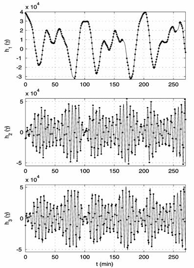
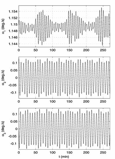
(a) (b)
Fig.
1. On the reconstruction of the spacecraft attitude motion in interval 13: (a)
the approximation of the magnetic field measurements, (b) the spacecraft
angular rate. The instant ![]() in the
plots corresponds to 09:21:20 UTC 09.06.2005,
in the
plots corresponds to 09:21:20 UTC 09.06.2005, ![]() ,
, ![]() deg./s,
deg./s, ![]() deg./s,
deg./s, ![]() deg./s,
deg./s, ![]() deg./s.
deg./s.
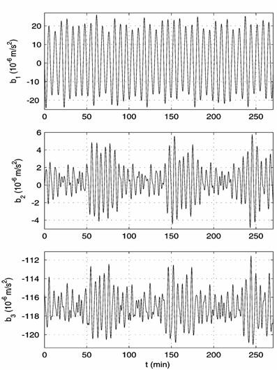
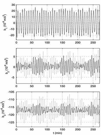
(a)
(b)
Fig.
2. The accelerations at the point of TAS3 location: (a) calculated for the
motion in interval 13 (Fig. 1), (b) measured by TAS3 (bold-faced lines shifted
to the left on ![]() s) and calculated for the motion in interval 13.
s) and calculated for the motion in interval 13.
(a)
(b)
Fig. 3. Elimination of the ultra low-frequency component from the filtered TAS3 measurements in interval 13:
(a) before elimination (fluent curves represent the ultra low-frequency component), (b) after elimination.

(a)
(b)
Fig.
4. The filtered acceleration component ![]() in interval
13; (a) the spectra, (b) the harmonic approximation and its error.
in interval
13; (a) the spectra, (b) the harmonic approximation and its error.
(a)
(b)
Fig.
5. The filtered acceleration component ![]() in
interval 13; (a) the spectra, (b) the harmonic approximation and its error.
in
interval 13; (a) the spectra, (b) the harmonic approximation and its error.
(a) (b)
Fig.
6. The calculated acceleration component ![]() in interval 13; (a)
the spectra, (b) the harmonic approximation and its error.
in interval 13; (a)
the spectra, (b) the harmonic approximation and its error.
(a)
(b)
Fig.
7. The calculated acceleration component ![]() in interval 13; (a)
the spectra, (b) the harmonic approximation and its error.
in interval 13; (a)
the spectra, (b) the harmonic approximation and its error.
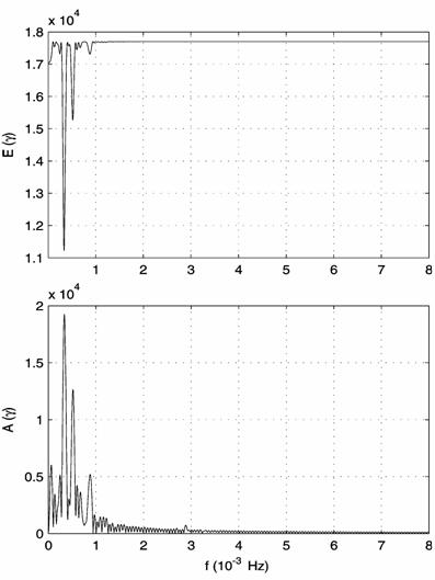
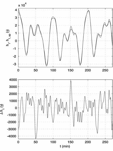
(a)
(b)
Fig.
8. The component ![]() of calculated strength
of the Earth magnetic field in interval 13;
of calculated strength
of the Earth magnetic field in interval 13;
(a)
the spectra, (b) the harmonic approximation and its error.
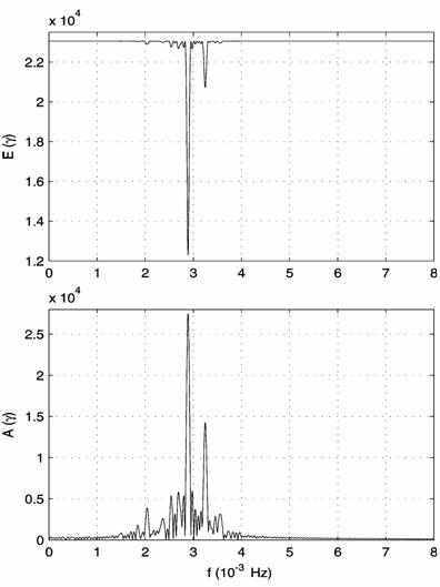
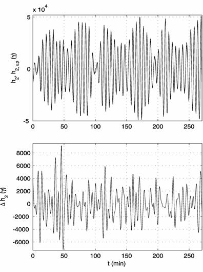
(a) (b)
Fig.
9. The component ![]() of calculated strength
of the Earth magnetic field in interval 13;
of calculated strength
of the Earth magnetic field in interval 13;
(a)
the spectra, (b) the harmonic approximation and its error.
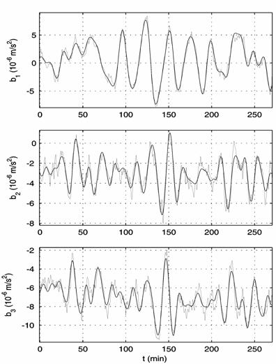
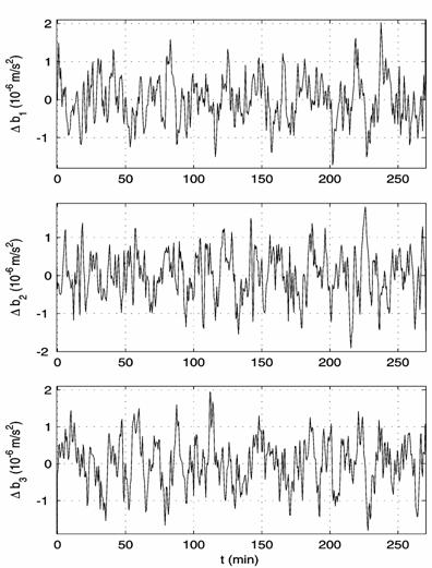
(a)
(b)
Fig. 10. The accelerations at the point of
TAS3 location in interval 2, ![]() m/s
m/s
![]() ;
;
(a) the corrected filtered functions ![]() and their calculated
analogs
and their calculated
analogs ![]() ,
(b) the differences
,
(b) the differences ![]()
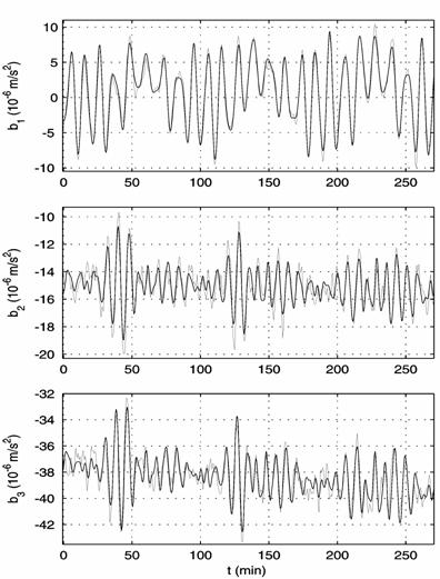
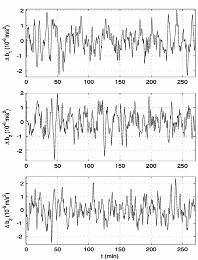
(a) (b)
Fig. 11. The accelerations at the point of
TAS3 location in interval 6, ![]() m/s
m/s![]() ;
;
(a) the corrected filtered functions ![]() and their calculated
analogs
and their calculated
analogs ![]() ,
(b) the differences
,
(b) the differences ![]() .
.
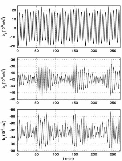
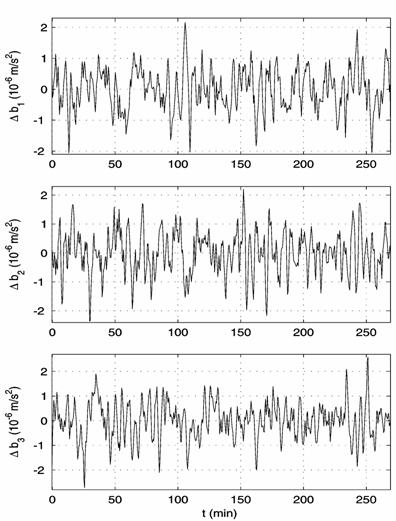
(a)
(b)
Fig. 12. The accelerations at the point of
TAS3 location in interval 13, ![]() m/s
m/s![]() ;
;
(a)
the corrected filtered functions ![]() and their calculated
analogs
and their calculated
analogs ![]() ,
(b) the differences
,
(b) the differences ![]() .
.