Design, building and experimental results of a facility to test hysteresis rod parameters
|
 .
. ,
,
|
Transformer |
|
|
Resistor
(Rp) |
|
|
Measured
Resistance of coil-1 |
|
|
Resistivity
of wire |
|
|
|
|
|
Section
of wire |
|
|
|
2342 |
|
Length
of wire for coil-1 |
|
|
|
|
|
|
|
|
|
|
|
Inductance
of coil-1 |
|
Fig.2. Facility during the realization (left) and
final assembling (right)
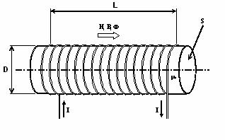
Number of loops for coil-1 has been chosen considering also that
solenoid had to cover whole length of hysteresis rod to evaluate rod parameters
changing position of the second coil. As a reference we considered for ![]() values variable from
values variable from ![]() and
and ![]() (
(![]() and
and ![]() ) on the Earth surface; value of Earth magnetic field in LEO
(Low Earth Orbit), for example at
) on the Earth surface; value of Earth magnetic field in LEO
(Low Earth Orbit), for example at ![]() of height, is
of height, is ![]() over the equator and
over the equator and ![]() over the poles.
Maximum value of magnetic field inside of the solenoid (
over the poles.
Maximum value of magnetic field inside of the solenoid (![]() ) is approximately
) is approximately ![]() . It corresponds to
. It corresponds to ![]() . In this case hysteresis rod is saturated. We can estimate
the intensity of saturation for the available rods for testing is approximately
. In this case hysteresis rod is saturated. We can estimate
the intensity of saturation for the available rods for testing is approximately
![]() . Using variable resistor the value of current which flows in
the solenoid and then the value of
. Using variable resistor the value of current which flows in
the solenoid and then the value of ![]() inside of coil-1 are
changed.
inside of coil-1 are
changed.
Fig.3. An example of hysteresis loop for a
ferromagnetic material (left). In the diagram the values of saturation and
coercitive fields for hysteresis rod-1 available for test in laboratory are
shown. The trend of magnetic permeability of a ferromagnetic material when B
changes is presented (right)
A typical hysteresis loop which shows the relation
between magnetizing field and induction for a ferromagnetic material is
available (Fig.3). Main notations are: ![]() is a saturation
induction,
is a saturation
induction, ![]() is a residual
induction,
is a residual
induction, ![]() is a coercitive force.
Shape of this cycle depends on an amplitude of
is a coercitive force.
Shape of this cycle depends on an amplitude of ![]() , material, its remagnetization history. Area inside of the
cycle is proportional to dissipated energy during a cycle [16]. In the right
the trend of magnetic permeability depending of
, material, its remagnetization history. Area inside of the
cycle is proportional to dissipated energy during a cycle [16]. In the right
the trend of magnetic permeability depending of ![]() is shown. The
permeability begins by an initial value which corresponds at inclination of
curve of first magnetization in the origin and grows until maximum value. After
that it decreases and inclines to the value of an initial permeability [16].
After such a brief summary of main parameters of the ferromagnetic material and
non-linearity of the magnetic permeability an idea of this experimental
activity is discussed.
is shown. The
permeability begins by an initial value which corresponds at inclination of
curve of first magnetization in the origin and grows until maximum value. After
that it decreases and inclines to the value of an initial permeability [16].
After such a brief summary of main parameters of the ferromagnetic material and
non-linearity of the magnetic permeability an idea of this experimental
activity is discussed.
Working principle of this facility is based on induction law of
Newman-Faraday-Lenz, that is, while a variable current flows in the coil-1 it
generates in a secondary coil an induced electromagnetic force. The secondary
coil (coil-2) is used as a sensor which moves along the solenoid (coil-1). We
see signals from coils on oscilloscope screen. Channel-1 of oscilloscope is
connected to the coil-1, channel-2 is connected to the coil-2. During the first
step of the work the idea is to observe Lissajous’s pictures (Appendix 1)
generated by these two signals and to establish the relation between
inclination of Lissajous’s ellipse which depends on difference of phase of two
signals and rod permeability along its length. Nevertheless, the non-linearity
of the ferromagnetic material (Fig.3) which composes the rod limits the
possibility to see a regular ellipse of Lissajous.
At the end of this section the problem of sizing of secondary coil and
choice of its placing with respect to the coil-1 is considered.
Magnetic field inside of coil-1 is calculated using the formulas [16]
 (2.3)
(2.3)
where the magnetic permeability of
vacuum ![]() is equal to
is equal to ![]() . Formulas (2.3) is valid for a solenoid with
. Formulas (2.3) is valid for a solenoid with ![]() (length of solenoid is
much more than radius of solenoid cross section) and not near extremities of
solenoid. Induced flux in the secondary coil is expressed by [16]
(length of solenoid is
much more than radius of solenoid cross section) and not near extremities of
solenoid. Induced flux in the secondary coil is expressed by [16]
![]() , (2.4)
, (2.4)
where ![]() is the magnetic field
induction inside of the coil-1,
is the magnetic field
induction inside of the coil-1, ![]() is a number of loops
of coil-2 and
is a number of loops
of coil-2 and ![]() is the cross section
of coil-2. Induced electromagnetic force in the coil-2 is evaluated on the
basis of the following set of formula [16]
is the cross section
of coil-2. Induced electromagnetic force in the coil-2 is evaluated on the
basis of the following set of formula [16]
 . (2.5)
Presence of factor ![]() reduces remarkably the amplitude
of signal of the coil-2 (≈mV). It means that it is important to evaluate
reduces remarkably the amplitude
of signal of the coil-2 (≈mV). It means that it is important to evaluate ![]() in way in order to get
a visible signal on the screen of the oscilloscope considering also the
presence of electromagnetic noise due to electrical network at
in way in order to get
a visible signal on the screen of the oscilloscope considering also the
presence of electromagnetic noise due to electrical network at ![]() within the laboratory.
To watch a signal on the channel-2 we fixed its amplitude
within the laboratory.
To watch a signal on the channel-2 we fixed its amplitude ![]() , that is,
, that is, ![]() and
and ![]() at least. On the basis
of this requirement the number of loops of coil-2 has been fixed at about 1500,
so that
at least. On the basis
of this requirement the number of loops of coil-2 has been fixed at about 1500,
so that ![]() . Test demonstrated that hysteresis rod amplifies this signal
in about 20 times. Main parameters of coil-2 are sketched in the Table 2.
. Test demonstrated that hysteresis rod amplifies this signal
in about 20 times. Main parameters of coil-2 are sketched in the Table 2.
Table 2. Main parameters of coil-2 of the facility for
testing of hysteresis rods magnetization
|
Measured
resistance of coil-2, |
|
|
Resistivity
of wire |
|
|
|
|
|
Cross
section |
|
|
|
1550 |
|
Length
of wire for coil-2 |
|
|
|
|
|
Section
of wire |
|
|
Inductance
of coil-2 |
|
The next step has been to establish the better way to arrange the
secondary coil with respect to the first coil to carry out measurements. Signal
of the coil-2 depends also on position of coil-2 with respect to the field
generated by coil-1. Signal is maximum when plane of the coils is perpendicular
to force lines of field generated by coil-1 and minimum while the plan is
parallel to the force lines. To maximize the factor of the mutual induction the
scheme of arrangement sketched in Fig.4 has been chosen.
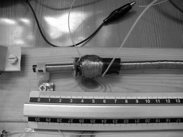
Fig.4. Scheme of arrangement of the coil-2 with
respect to the coil-1
To move coil-2 along the coil-1 in a very simple way we measure punctual
properties of the hysteresis rods placed inside of cylindrical support of
coil-1.
3. FIRST TEST OF THE FACILITY: EXISTENCE OF THE EARTH MAGNETIC FIELD AND
EFFECT OF HYSTERESIS RODS ON THE MAGNETIC FIELD INSIDE OF THE SOLENOID
A first elementary test has been performed to check functioning of the
facility. This test allowed us, also, to confirm variation of the rod
parameters along its length. A compass has been placed near the coil-1 without
to supply the facility and without a rod inside the core of solenoid. Magnetic
needle of compass finds one’s bearings in the magnetic north direction
(approximately 11.5 degrees far from geographic north direction). In this test
we are not interested in the quantitative results but qualitative analysis in
only. For this test it has been necessary to put a diode to supply facility
with a continue current because we need of a constant field which changes
direction of the compass needle. In this way we verify that facility works
generating a magnetic field inside of the solenoid. To do this a check
alimentation has been switched on. During this experience the value of variable
resistor was fixed at ![]() which corresponds to
which corresponds to ![]() . This value was comparable with value of Earth magnetic
field which lies on the Earth surface approximately in the range from
. This value was comparable with value of Earth magnetic
field which lies on the Earth surface approximately in the range from ![]() to
to ![]() . The compass needle did not change in a remarkable way but
to verify the correct working of facility it was enough to put one hysteresis
rod inside of core of solenoid: suddenly compass needle changed its position
moving of about 15 degrees. In the pictures 1 and 3 of Fig.5 one sees this
angular motion of the compass needle.
. The compass needle did not change in a remarkable way but
to verify the correct working of facility it was enough to put one hysteresis
rod inside of core of solenoid: suddenly compass needle changed its position
moving of about 15 degrees. In the pictures 1 and 3 of Fig.5 one sees this
angular motion of the compass needle.

Fig.5. First test of working of the facility
Moving hysteresis rod inside of coil-1 great variations of the angle
have been measured. This result confirmed the interest in the goal of this
work, that is, to try to explain in which way parameters of the hysteresis rod
change along its length and to develop a modelling useful for next applications
on board of small satellites.
4. SECOND TEST OF THE FACILITY: A RLC CIRCUIT TO VERIFY LISSAJOUS FIGURES
AT THE OSCILLOSCOPE SCREEN
A second test has been performed to check the instrumentation available
in the laboratory with aim to avoid uncertainties in the analysis of the
results of tests on the hysteresis rods during the next experimental activity.
The test has been carried out using a RLC circuit (Fig.6) with the main goal to
check Lissajous’s pictures visible on the screen of the oscilloscope depending
of different kind of signals in input. The part RC of circuit has been sized
(Appendix 2) in way to have two signals with the same amplitude to obtain a
Lissajous’s circle. Three resistances has been soldered in series in order to
obtain a total resistance of about ![]() . Capacitor has been chosen to obtain a signal with the same
amplitude (
. Capacitor has been chosen to obtain a signal with the same
amplitude (![]() ) of the resistance (
) of the resistance (![]() ). Its capacity is equal to
). Its capacity is equal to ![]() . As inductance has been chosen during the tests it has been
possible to establish that the coil-1 behaved as a resistance because its
inductance is very small. In fact a calculation of this inductance demonstrated
that its value is approximately equal to
. As inductance has been chosen during the tests it has been
possible to establish that the coil-1 behaved as a resistance because its
inductance is very small. In fact a calculation of this inductance demonstrated
that its value is approximately equal to ![]() , whereas its measured resistance is
, whereas its measured resistance is ![]() . In any case this fact did not restrict results of the test
because the idea was to use signals with different phases to confirm
theoretically expected Lissajous’s pictures and it was done with a RC circuit.
. In any case this fact did not restrict results of the test
because the idea was to use signals with different phases to confirm
theoretically expected Lissajous’s pictures and it was done with a RC circuit.
Fig.6. Circuit RLC used to test operative way X-Y in
the oscilloscope
Results obtained by connecting channel-1 of the oscilloscope with
resistance and channel-2 with capacitor are shown in Fig.7.
Amplitude of signal
is about the same (![]() and capacitive reactance
and capacitive reactance
![]() ) and they have a difference of phases of 90°.
) and they have a difference of phases of 90°.
Voltages ![]() and
and ![]() measured with oscilloscope
correspond at theoretical values. Corresponding Lissajous’s picture is an
ellipse very close to a circle with small disturbances.
measured with oscilloscope
correspond at theoretical values. Corresponding Lissajous’s picture is an
ellipse very close to a circle with small disturbances.
Fig.7. Results for RC circuit: signals with respect to
line (left) and corresponding Lissajous’s picture (right)
The same test has been carried out by connecting channel-1 and channel-2
of the oscilloscope with the same resistance. In this case Lissajous’s picture
expected is a line with an inclination of 45°. Results are visible in Fig.8.
Fig.8. Channel-1 and channel-2 connected at the same
signal in input
After, channel-1 has been connected with capacitor and channel-2 with
coil-1. Theoretically we exepect a difference of phases ![]() and Lissajous’s
picture is a line with an inclination of 135° but here this coil behaves as a
resistance because
and Lissajous’s
picture is a line with an inclination of 135° but here this coil behaves as a
resistance because ![]() . Results obtained with measurements confirm it (Fig.9).
. Results obtained with measurements confirm it (Fig.9).
Fig.9. Channel-1 connected at capacitor and channel-2
connected at coil-1
In Fig.8 we see two signals with ![]() where the second
signal has an amplitude quite less then one of the first signal (
where the second
signal has an amplitude quite less then one of the first signal (![]() and
and ![]() ). Correspondent Lissajous’s picture is an ellipse without
inclination with respect to axis X and Y. At the end, a test has been carried
out with a small inductance (
). Correspondent Lissajous’s picture is an ellipse without
inclination with respect to axis X and Y. At the end, a test has been carried
out with a small inductance (![]() ) and a resistance (
) and a resistance (![]() ). Result confirmed a difference of phase of 90°. These
simple tests allowed us to confirm a correct working of the oscilloscope (after
a compensation of the probes) and will be useful in the analysis of signal
related with hysteresis rods.
). Result confirmed a difference of phase of 90°. These
simple tests allowed us to confirm a correct working of the oscilloscope (after
a compensation of the probes) and will be useful in the analysis of signal
related with hysteresis rods.
5. THIRD TEST ON THE FACILITY: RESULTS OF TESTS WITHOUT RODS
It is well known [16] that in the extremities of a solenoid when a
current flows there is an edge effect which halves the value of internal field.
Neglecting values of field in the extremities of the solenoid (![]() ), measurements have been carried out from
), measurements have been carried out from ![]() of the length of the
solenoid to
of the length of the
solenoid to ![]() to verify the
uniformity of inducting field in the central part of the coil-1. Voltage
applied at the solenoid is
to verify the
uniformity of inducting field in the central part of the coil-1. Voltage
applied at the solenoid is ![]() corresponding to a
current
corresponding to a
current ![]() and to a field
and to a field ![]() inside of the coil-1.
Results available in Fig.10 show that there is not a very uniform behaviour of
internal field along the coil-1. Probably these results depend on non-uniform
distribution of coils during manufacturing process both coil-1 and coil-2. In
any case these results have to be taken into account in the analysis of the
measurements related to the hysteresis rods.
inside of the coil-1.
Results available in Fig.10 show that there is not a very uniform behaviour of
internal field along the coil-1. Probably these results depend on non-uniform
distribution of coils during manufacturing process both coil-1 and coil-2. In
any case these results have to be taken into account in the analysis of the
measurements related to the hysteresis rods.
Fig.10. Voltage values measured with coil-2 along the
solenoid without rod inside
6. RESULTS OF TESTS CARRIED OUT ON THE HYSTERESIS RODS
Tests have been performed on two different hysteresis rods. The first
rod named rod-1 has a length of ![]() and a section of
and a section of ![]() with a rectangular
shape. This type of rod has been utilized on board of MUNIN nanosatellite [10]
of Institute of Space Physics of Kiruna (Sweden) launched on 21th of
November, 2000 from Vandenberg Air Force Base located on the Central Coast of
California with the Delta 7000 Launch Vehicle. Rod-1 has been manufactured with
molybdenum permalloy of the 79NM specification; its composition includes 79% of
Ni, 4% of Mo and 17% of Fe [10]. Main parameters of the rod are available in
Table 3.
with a rectangular
shape. This type of rod has been utilized on board of MUNIN nanosatellite [10]
of Institute of Space Physics of Kiruna (Sweden) launched on 21th of
November, 2000 from Vandenberg Air Force Base located on the Central Coast of
California with the Delta 7000 Launch Vehicle. Rod-1 has been manufactured with
molybdenum permalloy of the 79NM specification; its composition includes 79% of
Ni, 4% of Mo and 17% of Fe [10]. Main parameters of the rod are available in
Table 3.
Table 3. Main
parameters of the rod
|
Initial magnetic permeability
|
Maximum magnetic permeability
|
Coercitive force
|
Residual
induction
|
Elongation of rod-1
|
|
25000 |
180000 |
1.6 |
0.74 |
250 |
Second hysteresis rod named rod-2 has a length of ![]() a section of
a section of ![]() with a rectangular
shape and elongation of p=65. For the rod main parameters are not available but
parameters of the material are available in [10, 17]. Information about
elongation allows us to do some considerations, that is, the parameter p for rod-2 is very far with respect to
the usual optimal values of elongation which lie in the range 200-300 [10]. In
our work for reasons of briefness and to give a complete view of the results
obtained with experimental tests of the rod-1 it will be refereed only diagrams
and results for this rod. Results of rod-2 confirm the same behaviour of the
rod-1. The shape of the signal is similar but much more irregularities appear
and values of amplitude are greater. Tests have been performed on the
hysteresis rod-1 changing the value of the current inside the coil-1. A summary
of some values is available in Table 4 where
with a rectangular
shape and elongation of p=65. For the rod main parameters are not available but
parameters of the material are available in [10, 17]. Information about
elongation allows us to do some considerations, that is, the parameter p for rod-2 is very far with respect to
the usual optimal values of elongation which lie in the range 200-300 [10]. In
our work for reasons of briefness and to give a complete view of the results
obtained with experimental tests of the rod-1 it will be refereed only diagrams
and results for this rod. Results of rod-2 confirm the same behaviour of the
rod-1. The shape of the signal is similar but much more irregularities appear
and values of amplitude are greater. Tests have been performed on the
hysteresis rod-1 changing the value of the current inside the coil-1. A summary
of some values is available in Table 4 where ![]() is the voltage applied
at coil-1,
is the voltage applied
at coil-1, ![]() is a current which
flows through the solenoid,
is a current which
flows through the solenoid, ![]() and
and ![]() are, respectively, the
magnetic field intensity and magnetic induction flux inside of the coil-1. In
the first case (
are, respectively, the
magnetic field intensity and magnetic induction flux inside of the coil-1. In
the first case (![]() ) rod is not in saturation. In the second one the rod
approaches the saturation. In the third case rod is in saturation. In the last
case we evaluated behaviour of the rod in a limit condition when
) rod is not in saturation. In the second one the rod
approaches the saturation. In the third case rod is in saturation. In the last
case we evaluated behaviour of the rod in a limit condition when ![]() (
(![]() is saturation field intensity).
is saturation field intensity).
Table 4. Main values of different configurations for test on the hysteresis rod-1
|
|
|
|
|
|
0.5 |
3.73 |
37.30 |
|
|
1.0 |
7.46 |
74.63 |
|
|
2.0 |
14.90 |
149.25 |
|
|
18.3 |
136.6 |
1366 |
|
For voltage values ![]() ,
, ![]() and
and ![]() it has been verified
that signal shape generated by coil-2 in the oscilloscope without rod inside of
the solenoid follows cosine law as it is evaluated in the relation (2.5)
assuming
it has been verified
that signal shape generated by coil-2 in the oscilloscope without rod inside of
the solenoid follows cosine law as it is evaluated in the relation (2.5)
assuming ![]() . The shape of signal related at the rod-1 when
. The shape of signal related at the rod-1 when ![]() and
and ![]() is sketched in Fig.11.
Preliminary results of measuring showed that the magnetic field is maximum in
the centre of the rods and minimum at the extremity and it should be noted that
there is no important changing in the shape (only in the amplitude) of the
signal when the position of the coil-2 varies along the rod-1. Tests have been
repeated with the facility arranged in a metallic box to verify if noise occurs
in these measurements but results obtained are the same.
is sketched in Fig.11.
Preliminary results of measuring showed that the magnetic field is maximum in
the centre of the rods and minimum at the extremity and it should be noted that
there is no important changing in the shape (only in the amplitude) of the
signal when the position of the coil-2 varies along the rod-1. Tests have been
repeated with the facility arranged in a metallic box to verify if noise occurs
in these measurements but results obtained are the same.
To confirm this result about magnetization of the rod tests have been
repeated with a different configuration (Fig.11). The goal was to check either
the field in the extremities of rod is in different times less with respect to
the value in the centre of rod due to the characteristics of magnetization
along the rod or this is an effect of the field in extremities of the solenoid
and an effect related to results showed in Fig.9.
Fig.11. Results of test on the hysteresis rod-1:
amplitude of signal is minimum at the extremities and maximum in the centre of
rod
In this configuration the coil-2 has been placed in different positions
along the solenoid and the rod has been inserted in way to do measurements at
its extremity. Scheme of this test with coil-2 arranged in the middle of
solenoid (at ![]() ) is shown in Fig.12. Results demonstrated that this trend can
be related to the characteristic of the magnetization of the rod.
) is shown in Fig.12. Results demonstrated that this trend can
be related to the characteristic of the magnetization of the rod.
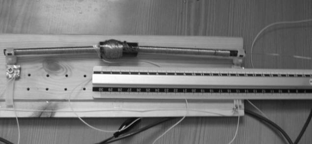
Fig.12. Results of test on the hysteresis rod-1:
coil-2 has been placed at 10 cm along the solenoid with respect to the left
extremity and hysteresis rod has been inserted in the coil-1 in a way to have
the left extremity inside of coil-2
Measurements have been completed by changing inclination
of coil-1 with respect to Earth magnetic field whose direction has been
specified with the compass. Measurements have been obtained for a random
inclination (Series-I: random ![]() ), in the perpendicular direction of coil-1 with respect to
Earth magnetic field direction (Series-II: normal
), in the perpendicular direction of coil-1 with respect to
Earth magnetic field direction (Series-II: normal ![]() ) and in the same direction of Earth magnetic field (Series-III:
parallel
) and in the same direction of Earth magnetic field (Series-III:
parallel ![]() ). In Fig.13, the diagram of the results obtained
with different set of measurements in laboratory is sketched.
). In Fig.13, the diagram of the results obtained
with different set of measurements in laboratory is sketched.
These results show that there is no a visible effect of the relative
position with respect to the Earth magnetic field direction. Small differences
in the measurements can depend on casual errors due to, for example, small
differences in the position of coil-2 along coil-1 or in the readings of
oscilloscope. When voltage applied to coil-1 increases the shape of signal
changes. This changing is visible in Fig.14. Results for hysteresis rod-1 when ![]() and
and ![]() are available in
Fig.15 and Fig.16 respectively.
are available in
Fig.15 and Fig.16 respectively.
Fig.13. Trend of magnetic field inside of rod-1: X
axis represents the length of hysteresis rod, Y axis represents experimentally
values obtained during tests in laboratory along the rod-1 for induced voltage
in coil-2. Diagram shows 3 set of measurements with different positions of the
facility with respect to Earth magnetic field direction
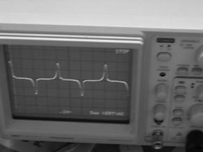
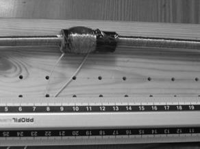
Fig.14. Results of test on the hysteresis rod-1: amplitude of
signal is maximum in the centre of rod; in this picture we see signal
corresponding at coil-2 placed at about 10.5 cm with respect to the extremity
of left of the rod when ![]()
Results for ![]() confirm the same
behaviour of these two previous cases. At this step of work we can not
establish if this changing depends by saturation of the rod or not. There are
not visible effects of the relative position between rod and Earth magnetic
field.
confirm the same
behaviour of these two previous cases. At this step of work we can not
establish if this changing depends by saturation of the rod or not. There are
not visible effects of the relative position between rod and Earth magnetic
field.
Fig.15.
Results for rod-1 for ![]() . Diagram shows three sets of measurements with different
positions of the facility with respect to Earth magnetic field direction
. Diagram shows three sets of measurements with different
positions of the facility with respect to Earth magnetic field direction
Fig.16.
Results for rod-1 for ![]() . Diagram shows three sets of measurements with different
positions of the facility with respect to Earth magnetic field direction
. Diagram shows three sets of measurements with different
positions of the facility with respect to Earth magnetic field direction
7. PRELIMINARY ANALYSIS OF THE SIGNALS
A number of mathematical models are available to describe the hysteresis
loop of soft magnetic material. We consider a simple approximating relation to
simulate magnetization curve of hysteresis [10]:
![]() (7.1)
(7.1)
where  . Here sign “+” is used for the ascending branch (right side
of the loop) and sign “–” is used for the descending portion (left side) of the
loop,
. Here sign “+” is used for the ascending branch (right side
of the loop) and sign “–” is used for the descending portion (left side) of the
loop,  ,
, ![]() is the coercitive
force,
is the coercitive
force, ![]() is the residual
induction of the rod and
is the residual
induction of the rod and ![]() is the saturation flux
density of permeable rod. Considering this approximation on the basis of
Newman-Faraday-Lenz law the following relation for induced signal in coil-2 is
obtained
is the saturation flux
density of permeable rod. Considering this approximation on the basis of
Newman-Faraday-Lenz law the following relation for induced signal in coil-2 is
obtained
 (7.2)
(7.2)
where ![]() and
and ![]() are the numbers of
loop of coil-1 and coil-2 respectively,
are the numbers of
loop of coil-1 and coil-2 respectively, ![]() is the length of
solenoid,
is the length of
solenoid, ![]() is the section of
coil-2,
is the section of
coil-2, ![]() (
(![]() ) is the pulsation and
) is the pulsation and ![]() is the amplitude of
current which flows through the solenoid. Graphic obtained by relation (7.2)
using MATLAB tools is available in Fig.17. In this relation all material
parameters are known except
is the amplitude of
current which flows through the solenoid. Graphic obtained by relation (7.2)
using MATLAB tools is available in Fig.17. In this relation all material
parameters are known except ![]() which is variable in
the range
which is variable in
the range ![]() for 4-79NM permalloy
[17]. Usually it can be estimated considering
for 4-79NM permalloy
[17]. Usually it can be estimated considering  for this material (it
means that
for this material (it
means that ![]() ) or evaluated from hysteresis loop (
) or evaluated from hysteresis loop (![]() ). Graphical representation shows that the signal shape
obtained using model (7.1) gives a good approximation for the signal shape
visible in the oscilloscope (while the road is in saturation) but the voltage
values are very different. This result depends on parameters
). Graphical representation shows that the signal shape
obtained using model (7.1) gives a good approximation for the signal shape
visible in the oscilloscope (while the road is in saturation) but the voltage
values are very different. This result depends on parameters ![]() ,
, ![]() and
and ![]() because we used
material parameters in this simulation (road parameters can be very different).
because we used
material parameters in this simulation (road parameters can be very different).
Fig.17. Mathematical results of signal in the
oscilloscope obtained considering
a simple approximating model
(7.1) for hysteresis
If we do not put
rod inside of the solenoid a mathematical relation which describes signal
induced in coil 2 is more simple and it follows a cosine law
 . (7.3)
On the basis of
this analysis we can conclude that the typical shape of signal obtained for
both rods depends on hysteresis properties. To confirm these results it is
necessary to repeat the tests on the others roads and to compare results.
Changing value of
current in the software used to simulate this signal a signal shape changes
simulating the signal shape in the oscilloscope. To try to obtain a better
analytical representation of the signal obtained during the tests in laboratory
when voltage ![]() and
and ![]() we changed empirically
the function (7.2). Using two parameters (
we changed empirically
the function (7.2). Using two parameters (![]() and
and ![]() ) a correct approximation for the shape of this signal has been obtained.
For amplitude it is necessary to multiply by a reduction factor
) a correct approximation for the shape of this signal has been obtained.
For amplitude it is necessary to multiply by a reduction factor ![]() because we used, in
this preliminary simulation, material parameters. Results of this first
empirical approximation while
because we used, in
this preliminary simulation, material parameters. Results of this first
empirical approximation while ![]() are available in
Fig.18. They can be compared with picture shown in Fig.11.
are available in
Fig.18. They can be compared with picture shown in Fig.11.
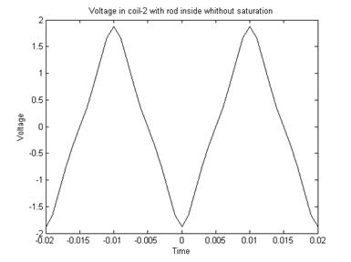
Fig.18. Analytical representation of measured
signal obtained using a simple mathematical model for hysteresis loop of rod-1,
![]() and introducing factors
and introducing factors ![]() and
and ![]() .
.
While current in the software is varied the shape of this function
changes as the signal in the oscilloscope. Results for ![]() and
and ![]() are visible in Fig.19.
are visible in Fig.19.
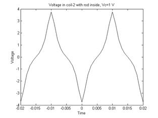

Fig.19.
Analytical
representation of measured signal obtained considering simple mathematical
model for hysteresis loop of rod-1, ![]() ,
for
,
for ![]() (left) and
(left) and ![]() (right)
(right)
8. CONCLUSIONS AND FUTURE PLAN
Due to certain limitations we do not have the possibility to expose all
experimental results obtained in the framework of this activity. In this first
part we described all phases of sizing and development of a facility to carry
out tests in laboratory on hysteresis rods. We described and showed tests carried
out to verify correct working of this facility and after that we showed test
results of the hysteresis rods. We verified experimentally that the magnetizing
field in the rod is maximum in the centre of the rod length and minimum in the
extremities. Changing the value of current inside of inducing coil (coil-1) we
verified hysteresis rod behaviour in different configurations: normal working,
approaching to the saturation and saturation. Effect of the relative position
between hysteresis rod and Earth magnetic field direction has been also
evaluated in all working conditions of the facility. In the last we determinate
an analytical representation of signal obtained using coil-2 when hysteresis
rod is arranged inside of the solenoid. This relation has been evaluated on the
basis of theoretical considerations for two simple models of the hysteresis but
it seems to approximate real signal shape only for values of current which
correspond to ![]() of the rod. To obtain
simulation of signal in normal working conditions of the rod and approaching to
the saturation we modified empirically previous relations. Comparison between
experimental results and pictures showed a good approximation but a more
accurate analysis to interpret behaviour of signal related to rod when voltage
applied to solenoid changes are requested. Tests to evaluate effects of a
permanent magnet on the hysteresis rods have been also carried out. The next
step of this work will be to interpret all experimental results and to try to
develop a modelling for the magnetic permeability of the rod depending by its
length.
of the rod. To obtain
simulation of signal in normal working conditions of the rod and approaching to
the saturation we modified empirically previous relations. Comparison between
experimental results and pictures showed a good approximation but a more
accurate analysis to interpret behaviour of signal related to rod when voltage
applied to solenoid changes are requested. Tests to evaluate effects of a
permanent magnet on the hysteresis rods have been also carried out. The next
step of this work will be to interpret all experimental results and to try to
develop a modelling for the magnetic permeability of the rod depending by its
length.
9. AKNOWLEDGEMENTS
The
work was supported by the Russian Foundation for Basic Research (Grants N
06-01-00389 and N 07-01-92001), the Program of the Leading Scientific Schools
Support (Grant N NSh-2448.2006.1) and Italian Space Agency.
REFERENCES
[1] V.A.Sarychev
and M.Yu. Ovchinnikov, Magnetic Attitude Control
Systems for Artificial Earth Satellites. Survey of Science and
Technology. Series: Exploration of Space, Moscow, 1985, VINITI, v.23, 104p.
[2] V.V.Beletskiy
and A.A.Khentov, Rotational Motion of a Magnetized Satellite. Moscow: Nauka. Main Office of
Physics and Mathematics Literature, 1985.
[3] M.Ovchinnikov, V.Pen'kov, O.Norberg and
S.Barabash, Attitude Control System for
the First Swedish Nanosatellite MUNIN, Acta Astronautica, 2000, V.46,
Issue 2-6, pp.319-326.
[4]
M.Yu.Ovchinnikov, V.I.Penkov, A.A.Ilyin and A.S.Selivanov, Magnetic Attitude Control Systems for the
Nanosatellite Series, Extended Abstracts for 5th International Symposium of
IAA "Small Satellites for Earth Observation", 4-8 April, 2005,
Berlin, Germany, Paper IAA-B5-1201,pp.429-432
[5] F.Graziani,
F.Santoni, F.Piergentili, F.Bulgarelli, M.Sgubini, M.Ronzitti, M.L.Battagliere, UNISAT microsatellites: an affordable way
to test in orbit innovative technologies and ideas, 23rd AIAA
International Communications Satellite Systems Conference, (ICSSC-2005), 25-28
Settembre, Roma
[6]
M.Yu.Ovchinnikov, A.A.Ilyin, N.V.Kupriyanova, V.I.Penkov, Attitude dynamics of the first Russian nanosatellite TNS-0, Acta
Astronauctica, 2007, Vol.61, Issue 1-6, 277-285
[7] F.Graziani, M.Ferrante, G.B.Palmerini, F.Santoni,
P.Tortora, UNISAT Program, a
University Tool for Space Education, paper IAF-00-P.2.07, 51st International Astronautical Congress,
2-6 Oct 2000, Rio de Janeiro, Brasil
[8] F.Santoni, M.Zelli, Passive Magnetic Attitute Stabilization of the Unisat-4 microsatellite,
57th
International Astronautical Congress, Valencia, Spain, 2-6th October 2006
[9] Ovchinnikov
M.Yu., Methods to Obtain the Principal
Parameters of Simple ACS for Small Satellites, Acta Astronautica, March
1998, V.43, Issue 11-12, pp.597-605
[10]
M.Yu.Ovchinnikov and V.I.Penkov, Passive
Magnetic Attitude Control System for the Munin Nanosatellite, Cosmic
Research, Vol.40, No. 2, 2002, pp 142-156
[11] A.P.Kovalenko, Magnetic Attitude
Control Systems of Space Vehicles,
M., Mechanical Engineering, 1975, 248 p
[12]
http://www.cubesatkit.com/
[13] M.Swartwout, University-Class Satellites: from marginal utility
to “Disruptive” Research Platforms, SSC04-II-5, 18th Annual
AIAA/USU, Conference on Small Satellites, Logan, UT, 9-12 August 2004
[14] M.Swartwout, Twenty (plus) year of University-Class
Spacecraft: a review of what was, an understanding of what is and look at what
should be next, 20th Annual AIAA/USU, August 2006
[15] V.A.Sarychev, V.I.Pen'kov, M.Yu.Ovchinnikov, Mathematical Model of a Hysteresis, Based
on Magnet-Mechanical Analogy, J. Matematicheskoe Modelirovanie, 1989, v.1,
N 4, pp.122-133
[16] D.Sette,
M.Bertolotti, Lezioni di Fisica 2:
Elettromagnetismo e ottica, Masson 1998, Milano, printed in Italy
[17] R.M.Bozort, Ferromagnetism, Van Nostrand Comapany,
Reinhold, New York 1951
APPENDIX 1: LISSAJOUS’S
FIGURES
Let us regard two simple harmonic motions and, at first, we consider
that they have the same frequency. We can chose origin of coordinate system to
have initial phase equal to zero along X axis; equation for ![]() coordinate is
coordinate is
![]() . (A.1.1)
. (A.1.1)
Equation for ![]() coordinate is
coordinate is
![]() , (A.1.2)
, (A.1.2)
where ![]() is the difference of
phase between oscillations
is the difference of
phase between oscillations ![]() and
and ![]() ,
, ![]() is the frequency of
signals and
is the frequency of
signals and ![]() and
and ![]() are the amplitudes; we
assume
are the amplitudes; we
assume ![]() . Trajectory of particle is limited by line of equation
. Trajectory of particle is limited by line of equation ![]() and
and ![]() . When
. When ![]() two motions are in
phase and equation of trajectory is
two motions are in
phase and equation of trajectory is
![]() . (A.1.3)
. (A.1.3)
This equation is represents by PQ in Fig.A.
Fig.A. Composition of simple harmonic motions with the
same frequency and perpendicular directions. Trajectory depends by difference
of phase of two signals
If ![]() then
then ![]() and equation of
trajectory is
and equation of
trajectory is
![]() . (A.1.4)
. (A.1.4)
This is equation is
represented by RS in Fig.A. It means that for![]() and
and ![]() we have a linear
polarization. If
we have a linear
polarization. If ![]() then
then ![]() , trajectory of particle is an ellipse with equation
, trajectory of particle is an ellipse with equation
 . (A.1.5)
Particle moves
along this ellipse in clockwise direction. To check this characteristic we
evaluate velocity of particle in the point A
![]() , (A.1.6)
, (A.1.6)
when ![]() (or
(or ![]() ) trajectory of particle is again an ellipse with axis
parallel to coordinate axes but particle moves along this in anticlockwise
direction. It means that for
) trajectory of particle is again an ellipse with axis
parallel to coordinate axes but particle moves along this in anticlockwise
direction. It means that for ![]() and
and ![]() there is an elliptical polarization in the composition of two
simple harmonic motions. If
there is an elliptical polarization in the composition of two
simple harmonic motions. If ![]() trajectory becomes a
circle and we say that there is a circular polarization for the composition of
two signals. For a generic value of
trajectory becomes a
circle and we say that there is a circular polarization for the composition of
two signals. For a generic value of ![]() trajectory is again an
ellipse but with axes inclined with respect to the coordinate axes. Changing
coordinate system one can demonstrate the relation between inclination of main
axes of ellipse with respect to coordinate axes
trajectory is again an
ellipse but with axes inclined with respect to the coordinate axes. Changing
coordinate system one can demonstrate the relation between inclination of main
axes of ellipse with respect to coordinate axes ![]() and
and ![]() difference of phase of
the two signal is
difference of phase of
the two signal is
![]() . (A.1.7)
. (A.1.7)
Some possible
trajectories for different ![]() (difference of phase)
are available in Fig.B. These trajectories are called Lissajous’s Figures.
(difference of phase)
are available in Fig.B. These trajectories are called Lissajous’s Figures.
Fig.B.
Possible trajectories for different ∆δ between two perpendicular
harmonic signals with the same frequency
Trajectory is an
enclosed curve while two signals have the same frequencies. If ![]() then the trajectory is
an open curve and shape of trajectory depends on the ratio
then the trajectory is
an open curve and shape of trajectory depends on the ratio ![]() and difference of
phase
and difference of
phase ![]() . Lissajous’s figures for different ratio
. Lissajous’s figures for different ratio ![]() and ∆δ are
sketched in Fig.C.
and ∆δ are
sketched in Fig.C.
Fig.C. Trajectories for different ![]() between two harmonic perpendicular signals
with different ratio
between two harmonic perpendicular signals
with different ratio![]()
APPENDIX
2: RLC CIRCUIT
Let us consider an RLC circuit supplied by an alternative voltage ![]() . Circuit equation is [16]
. Circuit equation is [16]
![]() . (A.2.1)
. (A.2.1)
This is a linear
differential equation similar to the equation of forced oscillations in a
mechanical system. Its solution is the sum of a homogenous solution of the
associate equation and of a particular integral. Homogenous solution describes
transitory. We are interested in the regime solution described by particular
integral. Particular solution is a current ![]()
![]() , (A.2.2)
, (A.2.2)
where ![]() is the difference of
phase and
is the difference of
phase and ![]() . To calculate
. To calculate ![]() and
and ![]() it needs to consider
the impedance
it needs to consider
the impedance ![]() of circuit. Then the
value of current is
of circuit. Then the
value of current is
 , (A.2.3)
where ![]() is the resistance,
is the resistance, ![]() is the inductive
reactance (
is the inductive
reactance (![]() , where
, where ![]() is the inductance) and
is the inductance) and
![]() is the capacitive
reactance (
is the capacitive
reactance (![]() , where
, where ![]() is the capacity). To
calculate the phase the following relation is used
is the capacity). To
calculate the phase the following relation is used
![]() . (A.2.4)
. (A.2.4)
Voltages for R, L
and C are
1)
![]()
2)
![]()
3)
![]()
APPENDIX
3: LIST OF SYMBOLS
![]() voltage
voltage
![]() voltage peak
(maximum amplitude)
voltage peak
(maximum amplitude)
![]() voltage peak to
peak
voltage peak to
peak
![]() current
current
![]() magnetic dipole
intensity
magnetic dipole
intensity
![]() number of loops of
coil-1
number of loops of
coil-1
![]() number of loops of
coil-1
number of loops of
coil-1
![]() cross section of
wire
cross section of
wire
![]() diameter of wire
diameter of wire
![]() diameter of cross
section of coil-1
diameter of cross
section of coil-1
![]() diameter of cross
section of coil-2
diameter of cross
section of coil-2
![]() length of coil-1
length of coil-1
![]() length of coil-2
length of coil-2
![]() length of wire for
coil 1
length of wire for
coil 1
![]() length of wire for
coil 2
length of wire for
coil 2
![]() resistivity of wire
resistivity of wire
![]() cross section of
coil-1
cross section of
coil-1
![]() cross section of
coil-2
cross section of
coil-2
![]() resistance of
potentiometer
resistance of
potentiometer
![]() resistance of
coil-1
resistance of
coil-1
![]() resistance of
coil-2
resistance of
coil-2
![]() magnetic field
induction
magnetic field
induction
![]() magnetic field intensity
magnetic field intensity
![]() Earth magnetic field intensity
Earth magnetic field intensity
![]() magnetic flux
magnetic flux
![]() induced
electromotive force
induced
electromotive force
![]() magnetic
permeability of vacuum
magnetic
permeability of vacuum
![]() capacitive
reactance
capacitive
reactance
![]() inductive reactance
inductive reactance
[1] Idea to
develop and build a laboratory facility for hyteresis rod parameters
exploration in combination with advanced numerical model was suggested by
Dr.Vladimir Pen’kov.