Physically Accurate Lighting Simulation in Computer Graphics Software

A.B. Khodulev, E.A. Kopylov

Contents Introduction Lightscape System Specter System Radiance System Scenes for Comparison Experimental Results Conclusion Acknowledgments

4. SCENES USED FOR COMPARISON

We used scenes of 3 classes for our comparison. The first class consists of only one simplest scene CUBE (interior of white diffusive cube illuminated by a point light source in its center) for which we can find accurate theoretical values of luminance distribution. It is important, because thus we can estimate absolute simulation accuracy of each system. The scene is described in more details in sec. 4.1.

The second class contains scenes originated from LVS. LVS is accompanied with some examples of scenes that demonstrate its possibilities. Unfortunately, we can not convert scenes in the internal LVS format to the other systems. Only one of the LVS examples, the scene ROOM, is present in DXF format, that can be converted. So, our second class consists of the single scene ROOM. It is a relatively simple scene. The scene presents an interior of a rectangular room with a table and 5 chairs around it. The room is illuminated by a square light source near the ceiling. All surfaces are diffusive. Their colors look artificially; it is probably caused by absence of attributes in DXF format. This scene is used for subjective comparison of image quality. Also we made an attempt to do quantitative comparison of simulation accuracy (see sec. 5.2).

The third class contains a more realistic (and more complex) examples of interiors. They are prepared by different companies and then converted to Specter format at Integra Inc. We used scenes in Specter format and converted them to other formats. For transformation to the Radiance format we developed a converter. Conversion to LVS was done via intermediate DXF format and then material attributes were assigned to LVS scene manually. These scenes were used only for visual comparison of image quality.

General information about all the scenes used is presented in the following table. Scene complexity is characterized by a number of triangles in a boundary representation.

Name	Created by	Triangles	Description	Figure
CUBE	Authors	12	Empty cube	1,2,4
ROOM	Lightscape	320	Room with chairs	3
APART2	Integra	5,000	An apartment	5
DREAM0	Korea National Housing	14,000	A living room	6
FLOWER	Voxel	17,000	A flower in a room	7
CG	Matsushita	32,000	A bathroom	8
HONSHA	Hibiya Engeneering	68,000	An office	9

Table 1. The scenes used for comparison.

4.1 Simple scene: an empty cube

The first scene used for comparison is simply an interior of a cube (10x10x10 m) with one point light source at its center (Fig.1). Luminous intensity of the light source is equal to 50000 cd that creates illumination level 2000 lux at nearest point on wall. The wall material is white with diffuse reflectivity 2/3 so that indirect component takes a great part in whole illumination.

Due to symmetry all the cube faces are equivalent. We've chosen several points on the cube face where theoretical results are compared with results produced by the systems being investigated. Although the scene is very simple, the exact analytical solution for illuminance distribution for it seems to be impossible. We used a combination of Monte Carlo simulation and direct numerical integration of the rendering equation to get accurate estimates of illuminance in a few selected points.

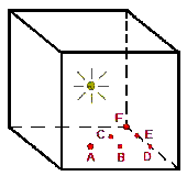
Fig.1. An empty cube.

Reference data

We analyzed luminance in several points on the cube face. These points constitute uniform 5x5 grid on the whole face. Due to symmetry there are only 6 different points (they are marked A-F in Fig. 1); they are presented in table 2 in local coordinates system: point (0, 0) is the face center, face edges have one +-1 coordinate. Below "semi-theoretical" luminance values for these points are presented. They are computed in the following way. At first we ran Monte Carlo simulation to get luminance distribution in cube faces. Then illuminance of each point was computed by direct integration of the energy transfer equation. This equation is equivalent to the rendering equation [Kaj86], for our case it can be written as:

$[Illum(p) = \int Lum(q) * cos(\alpha) * cos(\beta) / d(p, q)^2 dA(q) ]$ where

	Illum(p)	an unknown illuminance at some point p;
	Lum(q)	a luminance at point q;
		integral spans over all surface at scene;
		angles between the surface normal at point p and q and the segment connecting points p and q;
	r(p,q)	the Euclidian distance between p and q;
	dA(q)	the differential area element at point q.

A special trick was used to avoid singularity of this integral at the points lying on cube edges (the last 3 points in the table).

point	coordinate (x,y)	luminance (nit)	comment
A	(0, 0)	892.8	Face center
B	(0, 0.5)	768.7
C	(0.5, 0.5)	686.6
D	(0, 1)	565.1	Middle of edge
E	(0.5, 1)	522.4
F	(1, 1)	388.4	Cube corner

Table 2. The theoretical luminance values for the cube.

Actually we did not use all of these points in comparison; we used mainly the 3 points A, D, F as the most representative ones.

Contents Introduction Lightscape System Specter System Radiance System Scenes for Comparison Experimental Results Conclusion Acknowledgments


© Copyright 1996 Andrei B. Khodulev, Edward A. Kopylov.- All Rights Reserved	[Home]